Probabilistyczne anulowanie błędów z logicznymi modelami szumu

Szacowany czas: 28 minut na procesorze Heron r3 (UWAGA: To tylko szacunek. Twój rzeczywisty czas wykonania może się różnić.)

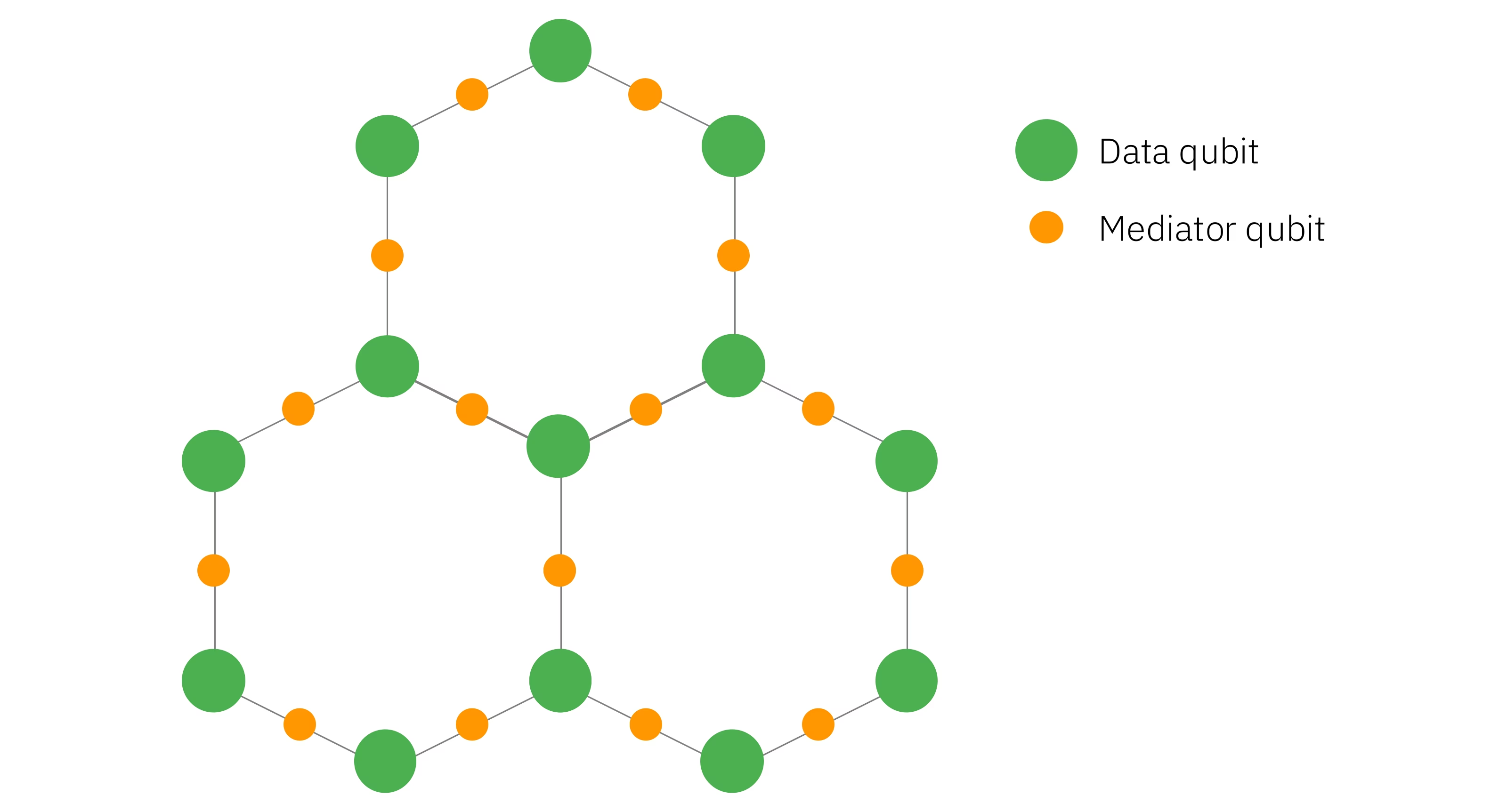In this tutorial we will evaluate observables of a 22-site Ising model on a hexagonal lattice using a Heron QPU, which has a heavy-hexagonal qubit topology. Many demonstrations on Heron QPUs focus on systems defined on heavy-hexagonal lattices to match the system's connectivity; however, hexagonal models tend to be more interesting to study as they appear more commonly in nature and are more difficult to simulate classically due to their denser connectivity. Since the qubit topology of the QPU cannot directly support the connectivity of a hexagonal lattice, we must decide how to efficiently embed the hexagonal model onto the qubit topology. In this example we represent each site in the Ising model with a qubit lying on a vertex of the heavy-hex QPU lattice. We use the qubits on the edges (mediator qubits) to facilitate entanglement between the Ising qubits on the vertices. Additionally, the mediator qubits implement entanglement in such a way that they are always expected to return to the ground state $|0\rangle$. If a mediator qubit measures $|1\rangle$, it indicates that a logical error occurred during circuit execution; postselecting only samples with no detected errors on the mediator qubits yields a smaller distribution of logical samples that might have a higher fidelity than the raw, noisy distribution. Not only can we detect that an error occurred by measuring a mediator qubit, we can also determine exactly which logical errors that qubit is capable of detecting throughout the circuit. Removing the noise generators the mediator qubits' symmetry checks are capable of detecting from a noise model leaves a reduced noise model, which can be mitigated using techniques such as probabilistic error cancellation (PEC).

W tym przykładzie notatnika połączymy opisaną powyżej technikę wykrywania błędów z PEC, aby skuteczniej przeciwdziałać szumowi kwantowemu niż każda z tych technik z osobna. Użyjemy 49 kubitów do osadzenia 22-kubitowego modelu Isinga oraz dodatkowych 27 kubitów mediatorowych do wykrywania błędów. Uruchomimy PEC na kanale szumu po postselekcji, aby ograniczyć szum, który umyka kontrolom symetrii. Oprócz połączenia wykrywania błędów z PEC, użyjemy technik takich jak łagodzenie błędów odczytu TREX oraz niemarkowowskie kontrole błędów, aby dodatkowo przeciwdziałać wpływowi szumu kwantowego.

Przebieg pracy jest następujący:

1. Symuluj klasycznie wartości oczekiwane obserwabli dla 22-kubitowego modelu hex-Isinga
2. Zaimplementuj 49-kubitowy model hex-Isinga wykrywający błędy za pomocą obwodu kwantowego i transpiluj go do backendu QPU
3. Określ warstwy splątujące w obwodzie za pomocą samplomatic. Nauczymy się szumu wpływającego na te warstwy splątujące i go złagodzimy.
4. Dodaj do obwodu niemarkowowskie kontrole błędów
5. Naucz się szumu bramek i odczytu wpływającego na obwód
6. Usuń z modelu szumu wyrazy wykrywane przez kontrole symetrii
7. Próbkuj obwód wykrywający błędy. Wybierz tylko próbki, które przechodzą wszystkie kontrole symetrii i niemarkowowskie kontrole błędów, oraz użyj łagodzenia odczytu TREX do wszystkich obliczeń wartości oczekiwanych
   • Próbkuj obwód wykrywający błędy
   • Próbkuj obwód wykrywający błędy z PEC, ale nie wybieraj próbek na podstawie kontroli symetrii i złagodź pełny wyuczony kanał szumu.
   • Próbkuj obwód wykrywający błędy z PEC. Wybierz próbki na podstawie kontroli symetrii i złagodź jedynie szum niewykrywalny przez kontrole.
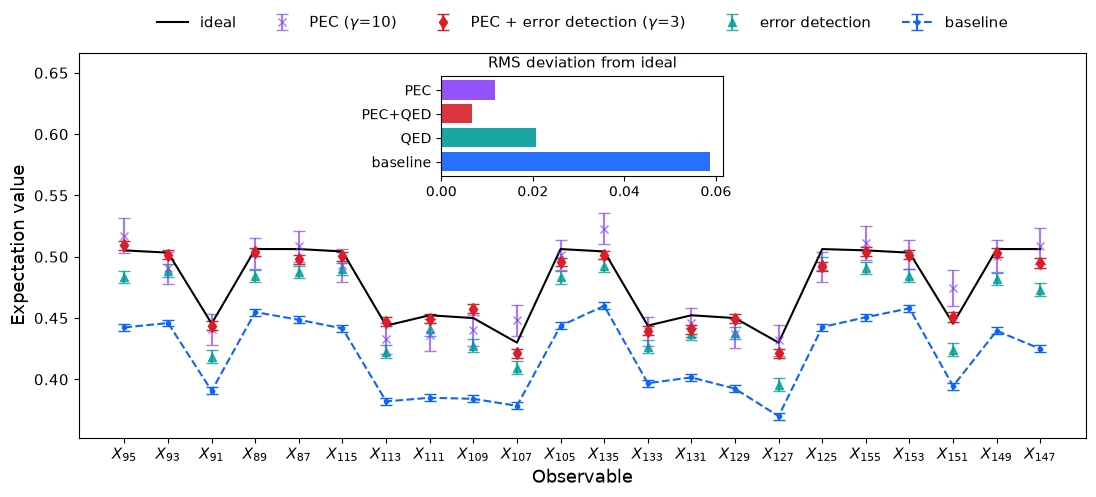
8. Oblicz wartości oczekiwane i porównaj strategie. Zaobserwuj, że QED+PEC skuteczniej anuluje szum wpływający na eksperyment niż każda z metod z osobna i daje zbieżne wartości oczekiwane przy znacznie mniejszej liczbie strzałów niż wymagane przez sam PEC.

Wymagania

Przed rozpoczęciem tego samouczka uruchom następujące polecenie, aby uzyskać wszystkie wymagane pakiety:

%pip install networkx numpy "qiskit[visualization]" "qiskit-ibm-runtime[visualization]" samplomatic qiskit-mitigation matplotlib "qiskit-noise-learning @ git+https://github.com/Qiskit/qiskit-noise-learning.git@ieee-demo-2026" Zwinięta komórka poniżej definiuje funkcje pomocnicze do rysowania wykresów używane w całym tym notatniku.

Kliknij, aby wyświetlić funkcje pomocnicze do rysowania wykresów

# Added by doQumentation — installs the packages this notebook needs if they are missing
import importlib.util

_needed = {"matplotlib": "matplotlib", "networkx": "networkx", "numpy": "numpy", "qiskit": "qiskit", "qiskit_ibm_runtime": "qiskit-ibm-runtime", "qiskit_mitigation": "qiskit-mitigation", "qiskit_noise_learning": "qiskit-noise-learning@git+https://github.com/Qiskit/qiskit-noise-learning.git@ieee-demo-2026", "samplomatic": "samplomatic"}
_missing = [pip for module, pip in _needed.items()
            if importlib.util.find_spec(module) is None]
# One at a time, so a package that fails to install does not block the others
for _pip in _missing:
    %pip install -q {_pip}
if not _missing:
    print("\u2713 All required packages are installed")

# Figure helpers for this notebook (collapsed): all plotting and styling lives here.
# The chip maps follow the style of Fig. 30 of arXiv:2607.25998.

from math import comb

import matplotlib.pyplot as plt
from matplotlib import cm
from matplotlib.colors import BoundaryNorm
from matplotlib.patches import Circle, Rectangle, Wedge

# one typography scheme for every figure in the notebook
plt.rcParams.update(
    {
        "font.size": 13,
        "axes.titlesize": 15,
        "axes.labelsize": 13,
        "xtick.labelsize": 11,
        "ytick.labelsize": 11,
        "legend.fontsize": 11,
    }
)

def x_labels(layout, n_data):
    """Per-observable tick labels carrying the physical qubit indices (site i = qubit i)."""
    return [f"$X_{{{layout[i]}}}$" for i in range(n_data)]

def plot_layout(backend, layout, n_data):
    """Chip cartoon of the embedding: data qubits green, check qubits orange."""
    from qiskit.visualization import plot_coupling_map

    return plot_coupling_map(
        num_qubits=backend.num_qubits,
        qubit_coordinates=None,
        coupling_map=list(backend.coupling_map.get_edges()),
        figsize=(9, 9),
        qubit_color=[
            "#4CAF50"
            if q in layout[:n_data]
            else "#FF9800"
            if q in layout[n_data:]
            else "#DDDDDD"
            for q in range(backend.num_qubits)
        ],
        qubit_size=220,
        line_width=2,
        font_size=90,
    )

def plot_exact(obs_exact, tick_labels, title):
    plt.figure(figsize=(12, 4))
    plt.plot(obs_exact, "o-")
    plt.title(title)
    plt.xticks(np.arange(len(obs_exact)), tick_labels)
    plt.xlabel("Observable")
    plt.ylabel(r"$\langle X \rangle$")
    plt.grid()

def draw_toy_circuit(
    generate_ed_ising, zz_coeff, x_coeff, include_checks=True
):
    """The boxing pipeline on a 3-plaquette-ring miniature (1 Trotter step) so the box
    structure is legible; every box carries the Twirl / InjectNoise annotations, and with
    ``include_checks`` the terminal xslow non-Markovian error check pattern is appended as in the
    production pipeline."""
    import networkx as nx
    from qiskit.circuit import ClassicalRegister
    from qiskit_mitigation.postselection import XSlowGate
    from samplomatic.transpiler import generate_boxing_pass_manager

    toy, _, _ = generate_ed_ising(nx.cycle_graph(3), 1, zz_coeff, x_coeff)
    toy.add_register(
        ClassicalRegister(3, "data"), ClassicalRegister(3, "check")
    )
    toy.barrier()
    toy.measure(range(3), range(3))
    toy.measure(range(3, 6), range(3, 6))
    toy_boxed = generate_boxing_pass_manager(
        enable_gates=True,
        enable_measures=True,
        inject_noise_targets="gates",
        inject_noise_strategy="individual_modification",
        inject_noise_site="after",
        twirling_strategy="active_circuit",
        measure_annotations="all",
    ).run(toy)
    if include_checks:
        toy_boxed.add_register(
            ClassicalRegister(3, "data_ps"), ClassicalRegister(3, "check_ps")
        )
        toy_boxed.barrier()
        for qb in range(6):
            toy_boxed.append(XSlowGate(), [qb])
        toy_boxed.measure(range(3), toy_boxed.cregs[2])
        toy_boxed.measure(range(3, 6), toy_boxed.cregs[3])
    return toy_boxed.draw("mpl", fold=-1, scale=0.6)

# --- chip-level noise maps ---------------------------------------------------------

BANDS = [1e-5, 2e-5, 3e-5, 4e-5, 6e-5, 1e-4, 2e-4, 3e-4, 4e-4, 6e-4, 1e-3]
CMAP = plt.get_cmap("YlOrBr")
NORM = BoundaryNorm(BANDS, CMAP.N, extend="both")

def _color(rate):
    return (
        "white"
        if rate < BANDS[0]
        else CMAP(NORM(min(rate, BANDS[-1] * 0.999)))
    )

def _layer_sparse(mit, weights):
    """Per-layer labelled terms from the saved run, box-local -> physical qubits."""
    phys = np.sort(mit["layout"])
    return [
        [
            (p, tuple(int(phys[q]) for q in qs if q >= 0), r)
            for p, qs, r in zip(
                mit[f"label_paulis_{i}"],
                mit[f"label_qubits_{i}"],
                w,
                strict=True,
            )
        ]
        for i, w in enumerate(weights)
    ]

def _aggregate(layers):
    """w1[qubit][P] and w2[(a,b)][PaPb]: rates summed over the 3 layers."""
    w1, w2 = {}, {}
    for terms in layers:
        for p, qs, r in terms:
            if len(qs) == 1:
                w1.setdefault(qs[0], dict.fromkeys("XYZ", 0.0))[p] += r
            else:
                (a, pa), (b, pb) = sorted(zip(qs, p, strict=True))
                w2.setdefault(
                    (a, b), {x + y: 0.0 for x in "XYZ" for y in "XYZ"}
                )[pa + pb] += r
    return w1, w2

def draw_noise_map(mit, backend, reduced=False):
    """Chip map of the learned model: X/Y/Z wheel per qubit, 3x3 two-qubit Pauli grid per
    coupler, log-banded colors, dashed outlines for unused hardware.

    With ``reduced=True``, keeps only the error terms the checks cannot see: detectability
    depends on circuit position, so each layer's 0/1 site scales are averaged over its uses.
    """
    from qiskit_ibm_runtime.visualization.embeddings import Embedding

    if reduced:
        scales = [
            mit["site_scales"][mit["site_layer"] == i].mean(axis=0)
            for i in range(3)
        ]
        weights = [mit[f"rates_{i}"] * scales[i] for i in range(3)]
        title = f"Reduced noise model ($\\gamma$ = {mit['gammas'][1]:.1f})"
    else:
        weights = [mit[f"rates_{i}"] for i in range(3)]
        title = f"Full noise model ($\\gamma$ = {mit['gammas'][0]:.0f})"
    w1, w2 = _aggregate(_layer_sparse(mit, weights))

    xy = np.array(
        [(c, -r) for r, c in Embedding.from_backend(backend).coordinates]
    )
    fig, ax = plt.subplots(figsize=(13, 7))
    for a, b in {tuple(sorted(e)) for e in backend.coupling_map.get_edges()}:
        if (
            (
                a,
                b,
            )
            in w2
        ):  # 3x3 Pauli grid laid along the bond (columns: qubit a, rows: qubit b)
            d = xy[b] - xy[a]
            u = d / np.hypot(*d)
            v = np.array([-u[1], u[0]])
            cl, cw = (np.hypot(*d) - 0.6) / 3, 0.17
            for i, Pa in enumerate("XYZ"):
                for j, Pb in enumerate("XYZ"):
                    ax.add_patch(
                        Rectangle(
                            xy[a] + u * (0.3 + i * cl) + v * ((j - 1.5) * cw),
                            cl,
                            cw,
                            angle=np.degrees(np.arctan2(u[1], u[0])),
                            facecolor=_color(w2[a, b][Pa + Pb]),
                            edgecolor="black",
                            lw=0.4,
                            zorder=2,
                        )
                    )
        else:
            ax.plot(
                *zip(xy[a], xy[b], strict=True),
                ls="--",
                lw=0.7,
                color="black",
                alpha=0.5,
                zorder=1,
            )
    for q, (xq, yq) in enumerate(xy):
        if q in w1:  # three-sector wheel: X top, Y lower left, Z lower right
            for P, t0 in (("X", 30), ("Y", 150), ("Z", 270)):
                ax.add_patch(
                    Wedge(
                        (xq, yq),
                        0.3,
                        t0,
                        t0 + 120,
                        facecolor=_color(w1[q][P]),
                        edgecolor="black",
                        lw=0.6,
                        zorder=3,
                    )
                )
            ax.annotate(
                str(q),
                (xq + 0.39, yq - 0.39),
                fontsize=9,
                color="gray",
                ha="left",
                va="top",
                zorder=4,
            )  # southeast, clear of the bond grids
        else:
            ax.add_patch(
                Circle(
                    (xq, yq),
                    0.24,
                    facecolor="none",
                    edgecolor="black",
                    ls="--",
                    lw=0.7,
                    alpha=0.5,
                    zorder=3,
                )
            )
    ux = xy[sorted(w1)]
    ax.set_xlim(ux[:, 0].min() - 2.2, ux[:, 0].max() + 2.2)
    ax.set_ylim(ux[:, 1].min() - 1.6, ux[:, 1].max() + 1.6)
    ax.set_aspect("equal")
    ax.axis("off")
    ax.set_title(title, fontsize=15)
    cb = fig.colorbar(
        cm.ScalarMappable(norm=NORM, cmap=CMAP),
        ax=ax,
        fraction=0.035,
        pad=0.02,
        extend="both",
        ticks=BANDS,
    )
    cb.set_label("coefficient (log bands; white < 1e-05)", fontsize=11)
    cb.ax.set_yticklabels(
        [f"{b:.0e}".replace("e-0", "e-") for b in BANDS], fontsize=10
    )
    _noise_map_legends(fig, ax)

def _noise_map_legends(fig, ax):
    """Weight-1 wheel and weight-2 grid keys, in a reserved band left of the lattice."""
    fig.subplots_adjust(left=0.17)
    axl = ax.inset_axes([-0.185, 0.70, 0.13, 0.24])
    for P, t0 in (("X", 30), ("Y", 150), ("Z", 270)):
        axl.add_patch(
            Wedge(
                (0.5, 0.45),
                0.38,
                t0,
                t0 + 120,
                facecolor="white",
                edgecolor="black",
                lw=0.8,
            )
        )
        axl.annotate(
            P,
            (
                0.5 + 0.2 * np.cos(np.radians(t0 + 60)),
                0.45 + 0.2 * np.sin(np.radians(t0 + 60)),
            ),
            ha="center",
            va="center",
            fontsize=9,
        )
    axl.set_title("weight-1", fontsize=10)
    axl.set_xlim(0, 1)
    axl.set_ylim(0, 1)
    axl.set_aspect("equal")
    axl.axis("off")
    axm = ax.inset_axes([-0.185, 0.32, 0.14, 0.30])
    for i, Pa in enumerate("XYZ"):
        for j, Pb in enumerate("XYZ"):
            axm.add_patch(
                Rectangle(
                    (i / 3, 1 - (j + 1) / 3),
                    1 / 3,
                    1 / 3,
                    facecolor="white",
                    edgecolor="black",
                    lw=0.6,
                )
            )
            axm.annotate(
                Pa + Pb,
                ((i + 0.5) / 3, 1 - (j + 0.5) / 3),
                ha="center",
                va="center",
                fontsize=7.5,
            )
        axm.annotate(Pa, ((i + 0.5) / 3, 1.08), ha="center", fontsize=8.5)
        axm.annotate(
            "XYZ"[i],
            (-0.13, 1 - (i + 0.5) / 3),
            ha="center",
            va="center",
            fontsize=8.5,
        )
    axm.annotate("qubit a", (0.5, 1.27), ha="center", fontsize=9)
    axm.annotate(
        "qubit b", (-0.33, 0.5), rotation=90, va="center", fontsize=9
    )
    axm.set_xlim(-0.35, 1.05)
    axm.set_ylim(-0.05, 1.35)
    axm.set_aspect("equal")
    axm.axis("off")

# --- run diagnostics ---------------------------------------------------------------

def plot_trex(trex_rescale, tick_labels):
    _fig, axt = plt.subplots(figsize=(12, 3))
    axt.stem(np.arange(len(trex_rescale)), (trex_rescale - 1) * 100)
    axt.set_xticks(np.arange(len(trex_rescale)), tick_labels)
    axt.set_xlabel("Observable")
    axt.set_ylabel("Readout correction (%)")
    axt.set_title("TREX rescale factors")
    plt.tight_layout()

def plot_postselection(mit):
    """Accepted shots per PEC randomization against a single binomial at the mean
    acceptance rate: agreement means acceptance is independent of the sampled circuit
    instance, the condition under which pooling accepted shots across randomizations
    is a consistent estimator."""
    _fig, ax = plt.subplots(figsize=(7.5, 3.8))
    counts = mit["acc_counts_post"]
    K, p = 64, counts.mean() / 64
    ks = np.arange(K + 1)
    pmf = np.array([comb(K, k) * p**k * (1 - p) ** (K - k) for k in ks])
    ax.hist(
        counts,
        bins=np.arange(-0.5, K + 1.5),
        density=True,
        alpha=0.6,
        color="#da1e28",
        label="measured",
    )
    ax.plot(ks, pmf, "k-", lw=1.5, label=f"Binomial(64, {p:.3f})")
    ax.set_xlim(-0.5, max(int(counts.max()) + 3, 20))
    ax.set_xlabel("Accepted shots per randomization")
    ax.set_ylabel("Probability")
    ax.legend()
    ax.grid(alpha=0.4)
    plt.tight_layout()

def plot_convergence(mit, obs_exact, n_data):
    """Running site-averaged estimate vs. randomizations for both PEC arms (the S5-consistent
    signed-ratio estimator, evaluated on growing prefixes of the sweep)."""

    def running(prefix):
        bits = np.squeeze(
            np.unpackbits(mit[f"data_{prefix}"], axis=-1)[..., :n_data]
            ^ mit[f"flips_{prefix}"]
        )
        mask = np.squeeze(mit[f"mask_{prefix}"])
        signs = 1 - 2 * (np.squeeze(mit[f"signs_{prefix}"]).sum(axis=-1) % 2)
        qv = (1 - 2 * bits.astype(int)) * mit["trex_rescale"]
        u = (
            (signs[:, None, None] * mask[..., None] * qv)
            .sum(axis=1)
            .mean(axis=1)
        )
        v = signs * mask.sum(axis=1)
        Rs = np.arange(500, len(u) + 1, 500)
        est, err = [], []
        for R in Rs:
            e = u[:R].sum() / v[:R].sum()
            est.append(e)
            err.append(
                np.sqrt(((u[:R] - e * v[:R]) ** 2).sum()) / abs(v[:R].sum())
            )
        return Rs, np.array(est), np.array(err)

    _fig, ax = plt.subplots(figsize=(12, 5))
    ideal_avg = float(np.mean(obs_exact))
    ax.axhline(ideal_avg, color="black", label="ideal")
    ax.fill_between(
        [-400, 24000],
        ideal_avg - 0.025,
        ideal_avg + 0.025,
        color="grey",
        alpha=0.22,
        label=r"$\pm 0.025$",
    )
    for prefix, label, color in (
        ("van", "vanilla PEC", "#8a3ffc"),
        ("post", "PEC + error detection", "#da1e28"),
    ):
        Rs, est, err = running(prefix)
        ax.errorbar(
            Rs,
            est,
            yerr=err,
            marker="o",
            linestyle="",
            markerfacecolor="none",
            color=color,
            alpha=0.85,
            capsize=3,
            label=label,
        )
    ax.set_xlim(-400, 24000)
    ax.set_ylim(ideal_avg - 0.08, ideal_avg + 0.08)
    ax.set_xlabel("# randomizations")
    ax.set_ylabel(r"Site-averaged $\langle X \rangle$")
    ax.legend(ncols=2)

def plot_final(
    obs_exact, baseline, ed, pec, post, gammas, tick_labels, title
):
    """Per-site <X> for every method, with an rms-deviation inset.
    baseline/ed/pec/post are (values, errors) pairs; gammas is (gamma, gamma_post)."""
    x = np.arange(len(obs_exact))
    _fig, ax = plt.subplots(figsize=(13, 5))
    h_ideal = ax.errorbar(
        x, obs_exact, fmt="-", capsize=4, label="ideal", color="black"
    )
    h_base = ax.errorbar(
        x,
        baseline[0],
        yerr=baseline[1],
        fmt=".--",
        capsize=4,
        label="baseline",
        color="#0f62fe",
    )
    h_ed = ax.errorbar(
        x,
        ed[0],
        yerr=ed[1],
        fmt="^",
        capsize=4,
        label="error detection",
        color="#009d9a",
        alpha=0.8,
    )
    h_pec = ax.errorbar(
        x,
        pec[0],
        yerr=pec[1],
        fmt="x",
        capsize=4,
        label=f"PEC ($\\gamma$={gammas[0]:.0f})",
        color="#8a3ffc",
        alpha=0.7,
    )
    h_post = ax.errorbar(
        x,
        post[0],
        yerr=post[1],
        fmt="d",
        capsize=4,
        label=f"PEC + error detection ($\\gamma$={gammas[1]:.0f})",
        color="#da1e28",
    )
    ax.set_xticks(x, tick_labels)
    ax.set_xlabel("Observable")
    ax.set_ylabel("Expectation value")
    # Set the y-axis range using the ideal, baseline, error detection, and PEC + error
    # detection curves, including error bars. Exclude PEC-only values when setting the
    # range so large fluctuations do not make the other curves difficult to distinguish.
    # PEC-only values may fall outside the visible range. Leave room above for the inset.
    series = [np.asarray(obs_exact)] + [
        np.asarray(v) + s * np.asarray(e)
        for v, e in (baseline, ed, post)
        for s in (-1, 1)
    ]
    lo, hi = min(a.min() for a in series), max(a.max() for a in series)
    span = max(hi - lo, 0.1)
    ax.set_ylim(lo - 0.1 * span, hi + 1.05 * span)
    # legend ordered to match the curves' vertical positions in the chart
    ax.legend(
        handles=[h_ideal, h_pec, h_post, h_ed, h_base],
        ncols=5,
        loc="lower center",
        bbox_to_anchor=(0.5, 1.02),
        frameon=False,
    )
    ax.set_title(title, pad=44)

    # inset: rows bottom-to-top so it reads top-to-bottom: PEC, PEC+ED, ED, baseline
    axi = ax.inset_axes([0.36, 0.68, 0.28, 0.26])
    methods = [
        ("baseline", baseline[0], "#0f62fe"),
        ("QED", ed[0], "#009d9a"),
        ("PEC+QED", post[0], "#da1e28"),
        ("PEC", pec[0], "#8a3ffc"),
    ]
    for k, (_nm, vals, color) in enumerate(methods):
        axi.barh(
            k,
            np.sqrt(np.mean((vals - np.array(obs_exact)) ** 2)),
            color=color,
            alpha=0.9,
        )
    axi.set_yticks(range(4), [m[0] for m in methods], fontsize=10)
    axi.set_title("RMS deviation from ideal", fontsize=11)
    axi.tick_params(labelsize=10)
    axi.patch.set_alpha(1.0)
    axi.set_zorder(5)

Symuluj klasycznie $\langle X \rangle_i$ dla każdego miejsca w 22-kubitowym modelu hex-Isinga

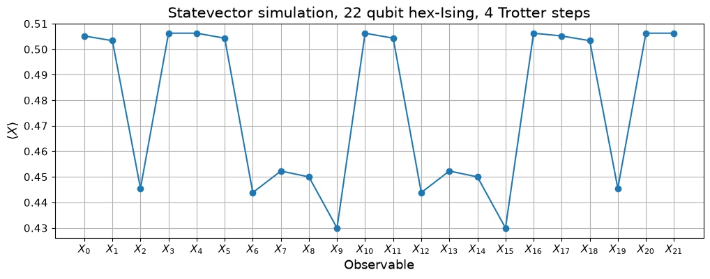
Najpierw używamy klasy Statevector z Qiskit, aby zasymulować dokładne wartości docelowe dla naszego eksperymentu. Chociaż rozwiązywany przez nas 22-kubitowy problem jest klasycznie rozwiązywalny, symulator statevector w Qiskit nie skaluje się do demonstracji dużo większych niż ta, a aby skalować się powyżej około 50 kubitów, musielibyśmy użyć niedokładnych technik symulacji, takich jak propagacja Pauliego. Ten 49-kubitowy eksperyment pozwala nam zbadać łączenie wykrywania błędów z łagodzeniem błędów na większą skalę, przy jednoczesnym zachowaniu dostępu do idealnych wartości oczekiwanych.

import warnings

import networkx as nx
import numpy as np
from qiskit.circuit import QuantumCircuit
from qiskit.quantum_info import Pauli, Statevector

# Silence two harmless upstream warnings (a Samplomatic default-change notice and a
# numpy datetime timezone notice from the noise-learning circuit generator)
warnings.filterwarnings(
    "ignore", message="The default of the 'inject_noise_site'"
)
warnings.filterwarnings(
    "ignore", message="no explicit representation of timezones"
)

# Hexagonal lattice
data_graph = nx.convert_node_labels_to_integers(
    nx.hexagonal_lattice_graph(2, 3)
)

# Number of Trotter steps and rotation angles
depth = 4
zz_coeff = -np.pi / 4
x_coeff = 3 * np.pi / 8
n_data = data_graph.order()
n_checks = data_graph.size()
n_qubits = n_data + n_checks

qc_data = QuantumCircuit(n_data)
qc_data.h(range(n_data))
for _ in range(depth):
    for edge in data_graph.edges:
        qc_data.rzz(zz_coeff, *edge)
    qc_data.rx(x_coeff, range(n_data))
psi_exact = Statevector(qc_data)

# X on site i = qubit i
observables = ["I" * (n_data - 1 - i) + "X" + "I" * i for i in range(n_data)]
obs_exact = [psi_exact.expectation_value(Pauli(o)).real for o in observables]

plot_exact(
    obs_exact,
    x_labels(range(n_data), n_data),
    f"Statevector simulation, {n_data} qubit hex-Ising, {depth} Trotter steps",
)

Zaimplementuj 49-kubitowy model hex-Isinga wykrywający błędy za pomocą obwodu kwantowego i transpiluj go do backendu QPU

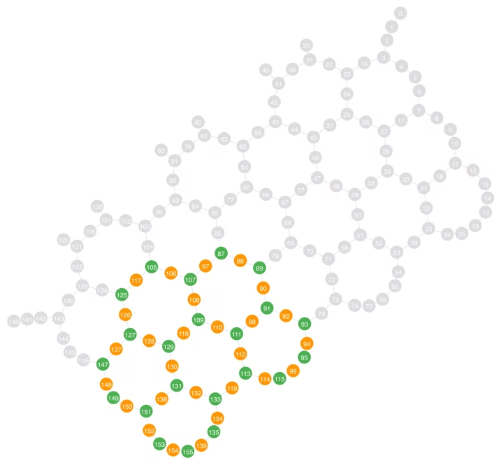
Ten obwód symuluje 4 kroki Trottera hamiltonianu Isinga z poprzecznym polem na sieci heksagonalnej dla 22 kubitów. 22 kubity danych są osadzone w 49-kubitowym podgrafie heavy-hex procesora QPU Heron r3, ibm_boston. 27 kubitów pomocniczych (ancilla) służy do dwóch celów: pośredniczenia w splątaniu między kubitami Isinga oraz wykrywania błędów logicznych podczas wykonywania obwodu. Warstwy splątujące obwodu są zaimplementowane tak, że kubity mediatorowe wracają do stanu podstawowego $|0\rangle$ przed swoimi końcowymi pomiarami. Zmierzenie stanu $|1\rangle$ przez jeden lub więcej kubitów mediatorowych wskazuje, że próbka została zniekształcona przez błąd logiczny. Odrzucenie tych próbek może poprawić wierność próbkowanego rozkładu.

Na poniższym grafie zielone kubity reprezentują 22 kubity Isinga, a pomarańczowe kubity reprezentują 27 kubitów mediatorowych.

from qiskit.circuit import ClassicalRegister
from qiskit.transpiler import generate_preset_pass_manager
from qiskit_ibm_runtime import QiskitRuntimeService

backend_name = "ibm_boston"

def generate_ed_ising(graph, depth, zz_coeff, x_coeff):
    """Build the mediated error-detecting Ising circuit for data-qubit `graph`; returns (circuit, CZ layers, hardware graph)."""
    hw_graph = nx.Graph()
    for i, (a, b) in enumerate(graph.edges()):
        hw_graph.add_edges_from(
            [(a, i + graph.order()), (b, i + graph.order())]
        )
    coloring = nx.coloring.greedy_color(
        nx.line_graph(hw_graph), strategy="DSATUR"
    )
    layers_coupling = [
        [e for e, c in coloring.items() if c == i]
        for i in set(coloring.values())
    ]
    circuit = QuantumCircuit(hw_graph.order())
    circuit.h(range(hw_graph.order()))
    for _ in range(depth):
        for angle, qubits in (
            (zz_coeff, range(graph.order(), hw_graph.order())),
            (x_coeff, range(graph.order())),
        ):
            circuit.barrier()
            for layer in layers_coupling:
                for edge in layer:
                    circuit.cz(*edge)
            circuit.barrier()
            circuit.rx(angle, qubits)
    circuit.barrier()
    circuit.h(range(graph.order(), hw_graph.order()))
    return circuit, layers_coupling, hw_graph

service = QiskitRuntimeService()
backend = service.backend(backend_name)

circuit, layers_coupling, hw_graph = generate_ed_ising(
    data_graph, depth, zz_coeff, x_coeff
)

circ_meas = circuit.copy()
data_reg, check_reg = (
    ClassicalRegister(n_data, "data"),
    ClassicalRegister(n_checks, "check"),
)
circ_meas.add_register(data_reg, check_reg)
circ_meas.barrier()
circ_meas.measure(range(n_data), data_reg)
circ_meas.measure(range(n_data, n_qubits), check_reg)

# Physical qubits hosting the 22 Ising sites on ibm_boston, one heavy-hex row per lattice chain;
# the mediator for each edge is the physical qubit sitting between its two data qubits
data_layout = [
    *[95, 93, 91, 89, 87],
    *[115, 113, 111, 109, 107, 105],
    *[135, 133, 131, 129, 127, 125],
    *[155, 153, 151, 149, 147],
]
coupling_graph = nx.Graph(list(backend.coupling_map.get_edges()))
layout = data_layout + [
    next(
        iter(
            nx.common_neighbors(
                coupling_graph, data_layout[a], data_layout[b]
            )
        )
    )
    for a, b in data_graph.edges()
]

circ_trans = generate_preset_pass_manager(
    backend=backend, optimization_level=1, initial_layout=layout
).run(circ_meas)

plot_layout(backend, layout, n_data)

Określ warstwy splątujące w obwodzie za pomocą samplomatic.

Przebieg generate_boxing_pass_manager z Samplomatic grupuje warstwy splątujące obwodu w opatrzone adnotacjami bloki na potrzeby Pauli twirling i wstrzykiwania szumu PEC. Wynikowy obwód szablonowy oraz samplex (rozkład parametryczny nad obwodem szablonowym, określający jego twirle i wstrzykiwanie szumu) są używane do zdefiniowania i wykonania wszystkich eksperymentów QPU związanych z uczeniem się szumu i próbkowaniem. Bloki pomiarowe niosą również adnotację ChangeBasis, dzięki czemu rotacje mierzące kubity danych w bazie X są dostarczane do samplexu jako dane wejściowe w momencie próbkowania, zamiast być wbudowane w obwód na stałe.

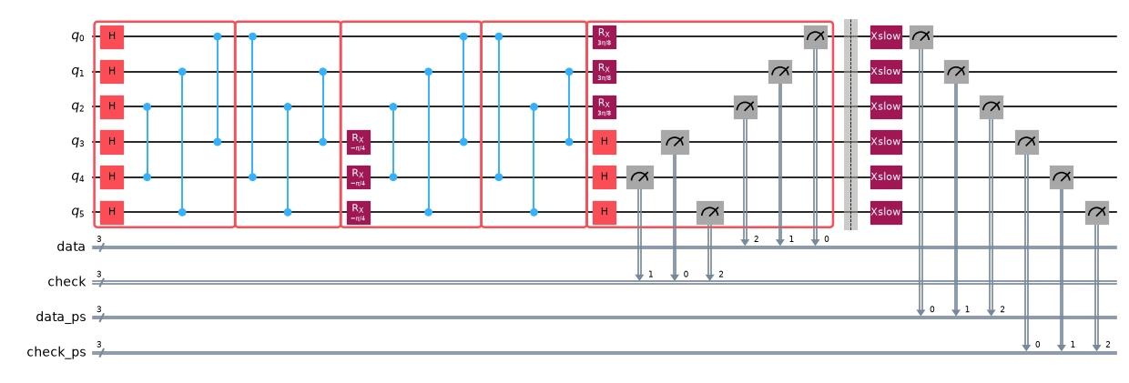
Poniżej ten sam przebieg boxingu jest zastosowany do niewielkiej wersji obwodu Isinga wykrywającego błędy, abyśmy mogli zwizualizować strukturę obwodu podzielonego na bloki.

from samplomatic.builders import build
from samplomatic.transpiler import generate_boxing_pass_manager
from samplomatic.utils import find_unique_box_instructions

boxed = generate_boxing_pass_manager(
    enable_gates=True,
    enable_measures=True,
    inject_noise_targets="gates",
    inject_noise_strategy="individual_modification",
    inject_noise_site="after",
    twirling_strategy="active_circuit",
    measure_annotations="all",
).run(circ_trans)
template, samplex = build(boxed)
unique_instructions = find_unique_box_instructions(
    boxed, normalize_annotations=None, undress_boxes=True
)

# Measure X on the data qubits and Z on the mediators
basis_key = next(
    s.name
    for s in samplex.inputs().get_specs()
    if s.name.startswith("basis_changes.")
)
meas_basis = np.array(
    [2 if q in set(layout[:n_data]) else 1 for q in sorted(layout)],
    dtype=np.uint8,
)

draw_toy_circuit(generate_ed_ising, zz_coeff, x_coeff, include_checks=False)

Dodaj do obwodu niemarkowowskie kontrole błędów

Następnie dodajemy do obwodu niemarkowowskie kontrole błędów, aby zabezpieczyć się przed szumem, który nie jest modelowany w naszym protokole uczenia. Kontrole te działają poprzez zaimplementowanie długiego impulsu odwracającego bit (bit-flip) i sprawdzenie, czy kubit poprawnie przeszedł z jednego stanu klasycznego do drugiego. Jeśli oba kubity na krawędzi nie przejdą kontroli, próbka jest odrzucana. Niemarkowowskie kontrole błędów mogą być stosowane na początku lub na końcu obwodu (lub w obu miejscach); tutaj używamy ich tylko na końcu. Umieszczamy również kontrole na nieużywanych kubitach-obserwatorach (ang. spectator qubits) sąsiadujących z obwodem, co pozwala lepiej wykrywać szum, do którego wykrywania te kontrole są przeznaczone.

Pamiętaj, że podobnie jak kontrole symetrii, jest to również forma postselekcji, więc musimy uwzględnić spadek współczynnika postselekcji przy łączeniu tych technik. Konkretnie, jeśli $P(\text{błąd niemarkowowski}) = \alpha$ i $P(\text{błąd symetrii}) = \beta$, to potrzeba w przybliżeniu $\frac{1}{(1-\alpha)(1-\beta)}$ zaszumionych próbek, aby odzyskać jedną próbkę logiczną.

from qiskit.transpiler import PassManager
from qiskit_mitigation.postselection import PostSelector
from qiskit_mitigation.postselection.passes import (
    AddPostCircuitNonMarkovianErrorChecks,
    AddSpectatorPostCircuitNonMarkovianErrorChecks,
)

add_checks = PassManager(
    [
        AddPostCircuitNonMarkovianErrorChecks(x_pulse_type="xslow"),
        AddSpectatorPostCircuitNonMarkovianErrorChecks(
            backend.coupling_map, x_pulse_type="xslow"
        ),
    ]
)
template_checked = add_checks.run(template)
selector = PostSelector.from_circuit(template_checked, backend.coupling_map)

draw_toy_circuit(generate_ed_ising, zz_coeff, x_coeff, include_checks=True)

Naucz się szumu bramek i odczytu dla 49-kubitowego kontrolowanego obwodu Isinga

Aby złagodzić szum, musimy zamodelować, w jaki sposób szum wpływa na nasze bramki splątujące. Tutaj uczymy się modelu szumu Pauliego-Lindblada dla każdej z trzech różnych warstw splątujących obwodu, używając qiskit-noise-learning. Później usuniemy z tego modelu szumu generatory błędów wykrywalne przez kontrole symetrii i złagodzimy za pomocą PEC tylko pozostały kanał szumu. Poniższa mapa pokazuje trzy wyuczone warstwy na procesorze QPU; każdy kubit to koło jego współczynników X/Y/Z wagi 1, a każdy sprzęgacz to siatka 3×3 współczynników Pauliego wagi 2 dla tej pary. Wartość $\gamma$ równa $10$ oznacza narzut próbkowania równy $\gamma^2=10^2=100$.

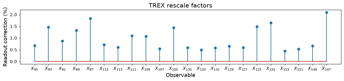
Poprawki odczytu (TREX) pochodzą bezpośrednio ze ścieżek SPAM dopasowania uczenia szumu. Wykres typu stem (pionowe słupki z punktami) poniżej mapy szumu QPU pokazuje współczynniki przeskalowania TREX dla poszczególnych obserwabli.

from qiskit.quantum_info import PauliLindbladMap, QubitSparsePauli
from qiskit_ibm_runtime import Executor, Session
from qiskit_ibm_runtime.quantum_program import QuantumProgram
from qiskit_mitigation.trex import TREX
from qiskit_noise_learning.analysis import (
    ComputeObservables,
    CurveFitObservables,
    FlipPostSelect,
    LeastSquaresSolve,
)
from qiskit_noise_learning.circuit_generator import ExecutorCircuitGenerator
from qiskit_noise_learning.experiment_builder import (
    BindFragmentDepths,
    CompleteSequences,
    EvenDepthVanillaPaths,
    Experiment,
    GenerateInstructionSequences,
    IdentifyRelations,
    MergeInstructionSequences,
    SPAMPaths,
    VanillaInstructionSequences,
)
from qiskit_noise_learning.gate_sets import QiskitGateSet
from qiskit_noise_learning.models import PauliLindbladModel
from qiskit_noise_learning.models.utils import split_pauli_lindblad_model
from samplomatic.annotations import InjectNoise
from samplomatic.utils import get_annotation

gate_set = QiskitGateSet(
    target=backend.target,
    qubit_subset=sorted(
        {
            boxed.find_bit(q).index
            for i in unique_instructions
            for q in i.qubits
        }
    ),
)
ref_to_qubits = {}
for inst in unique_instructions:
    if ann := get_annotation(inst.operation, InjectNoise):
        gate_set.add_box_as_gate(inst, name=ann.ref)
        ref_to_qubits[ann.ref] = sorted(
            boxed.find_bit(q).index for q in inst.qubits
        )

fidelity_model = PauliLindbladModel.k_local(
    gate_set, gate_k={**{r: 2 for r in ref_to_qubits}, "M": 1, "P": 1}
)
experiment = (
    EvenDepthVanillaPaths()
    + VanillaInstructionSequences()
    + IdentifyRelations()
    + SPAMPaths()
    + GenerateInstructionSequences()
    + MergeInstructionSequences()
    + CompleteSequences()
    + BindFragmentDepths([2, 4, 8, 12])
).run(Experiment(fidelity_model=fidelity_model, shots=384, randomizations=64))

circuit_generator = ExecutorCircuitGenerator(
    gate_set, pass_manager=add_checks
)
program_learn, data_mapper = circuit_generator.generate(experiment)

session = Session(backend)
executor_options = {"environment": {"job_tags": ["TUT_PECLNM"]}}
fit = circuit_generator.collect(
    Executor(session, options=executor_options).run(program_learn).result(),
    data_mapper,
)
fit = (
    FlipPostSelect()
    + ComputeObservables()
    + CurveFitObservables()
    + LeastSquaresSolve()
).run(fit)
print(
    "learning shots removed by checks:",
    f"{float(fit.raw_data.datatree['0']['data_mask'].mean()):.4f}",
)

# TREX factors from the fit's SPAM paths: the fit only identifies the product of
# state-prep and measurement error, so hand TREX the composition of the two maps
spam = fidelity_model.to_pauli_lindblad_maps(
    fit.model_data, include_spam=True
)
spam_map = spam["P"].compose(spam["M"])
z_terms = [
    QubitSparsePauli(("Z", [layout[i]]), num_qubits=backend.num_qubits)
    for i in range(n_data)
]
trex_rescale = np.array(
    [TREX.calculate_trex_factor(spam_map, z) for z in z_terms]
)

# learned maps come back in backend qubit indexing; samplex wants box-local order
plm = split_pauli_lindblad_model(fit.model).model
noise_maps = {}
for ref, m in plm.to_pauli_lindblad_maps(fit.model_data).items():
    box = ref_to_qubits[ref]
    noise_maps[ref] = PauliLindbladMap.from_sparse_list(
        [
            (p, tuple(box.index(q) for q in qs), r)
            for p, qs, r in m.to_sparse_list()
        ],
        num_qubits=len(box),
    )
# Full-PEC cost: each learned layer acts twice per Trotter step (compute + uncompute)
gamma = float(
    np.exp(2 * depth * sum(2 * sum(m.rates) for m in noise_maps.values()))
)

# Collect the learned model in the form the figure helpers expect
mit = dict(
    **{
        f"rates_{i}": np.asarray(m.rates)
        for i, m in enumerate(noise_maps.values())
    },
    **{
        f"label_paulis_{i}": np.array([p for p, _, _ in m.to_sparse_list()])
        for i, m in enumerate(noise_maps.values())
    },
    **{
        f"label_qubits_{i}": np.array(
            [
                list(qs) + [-1] * (2 - len(qs))
                for _, qs, _ in m.to_sparse_list()
            ]
        )
        for i, m in enumerate(noise_maps.values())
    },
    layout=np.array(layout),
    trex_rescale=trex_rescale,
    gammas=np.array([gamma, np.nan]),
)
draw_noise_map(mit, backend)
plot_trex(mit["trex_rescale"], x_labels(layout, n_data))

learning shots removed by checks: 0.2393

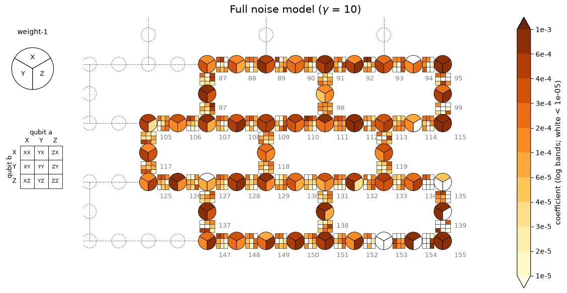
Usuń z modelu szumu wyrazy wykrywalne przez kontrole symetrii

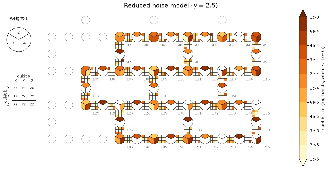
Każda kontrola symetrii jest w stanie wykryć pewien podzbiór generatorów błędów w modelu szumu, co oznacza, że nie trzeba łagodzić tych błędów. Tutaj tworzymy maskę nad wykrywalnymi generatorami szumu, używając funkcji create_postselected_noise_mask z qiskit_mitigation. Ta maska zostanie użyta do usunięcia z modelu szumu wykrywalnych wyrazów przed wykonaniem PEC. Wykonanie PEC względem oczyszczonego modelu szumu może dać zbieżne wartości oczekiwane za ułamek kosztu próbkowania wymaganego do wykonania PEC na pełnym modelu szumu, jak pokazano na powyższych mapach modelu szumu.

Poniższa mapa jest narysowana w tej samej skali kolorów co powyższy wyuczony model, zachowując jedynie generatory błędów, których kontrole nie są w stanie wykryć. Widzimy, że z modelu usunięto dużą liczbę generatorów błędów, a narzut próbkowania znacznie się zmniejszył. Narzut próbkowania potrzebny do uruchomienia PEC na oczyszczonym modelu szumu wynosi $\gamma^2=2.5^2\approx6.3$, co stanowi około 16-krotną redukcję w porównaniu z narzutem wymaganym do złagodzenia pełnego kanału szumu.

from qiskit.quantum_info import Pauli
from qiskit_mitigation.noise import create_postselected_noise_mask

SHOTS_PER_RAND = 64  # shots per PEC randomization
N_RAND = 23_054  # PEC randomizations per experiment
MAX_PAIR_RATE = 0.02  # Max value of any coupler's summed two-qubit error rate

# The detectors are virtual Pauli-Z's representing the measurements on the mediator qubits
# We can find the set of detectable noise generators in the model for each detector by conjugating
# it backward through the circuit and calculating what generators it anti-commutes with.
detectors = [
    Pauli("I" * (boxed.num_qubits - 1 - q) + "Z" + "I" * q)
    for q in layout[n_data:]
]
# Detectable generators are handled by postselection; prune them from the model for PEC
local_scales, gamma2_post = create_postselected_noise_mask(
    boxed, noise_maps, detectors
)
gamma_post = gamma2_post**0.5
print(f"gamma PEC {gamma:.2f} | gamma QED+PEC {gamma_post:.2f}")

# Kill the job if any coupler's summed rate exceeds MAX_PAIR_RATE
pair_lam = {}
for m in noise_maps.values():
    for _, qs, r in m.to_sparse_list():
        if len(qs) == 2:
            pair_lam[tuple(sorted(qs))] = (
                pair_lam.get(tuple(sorted(qs)), 0.0) + r
            )
assert (
    max(pair_lam.values()) < MAX_PAIR_RATE
), f"kill: degraded coupler {max(pair_lam, key=pair_lam.get)}"

# Detectability depends on circuit position, so record each site's 0/1 scales by layer
site_ref = {
    a.modifier_ref: a.ref
    for inst in boxed.data
    if inst.operation.name == "box"
    and (a := get_annotation(inst.operation, InjectNoise))
    and a.ref
}
sites = sorted(local_scales, key=lambda s: int(s[1:]))
mit["site_scales"] = np.stack([local_scales[s] for s in sites])
mit["site_layer"] = np.array(
    [list(noise_maps).index(site_ref[s]) for s in sites]
)
mit["gammas"] = np.array([gamma, gamma_post])
draw_noise_map(mit, backend, reduced=True)

gamma PEC 10.08 | gamma QED+PEC 2.52

Próbkuj obwód wykrywający błędy

Tutaj próbkujemy 49-kubitowy obwód Isinga wykrywający błędy. Włączamy Pauli twirling oraz niemarkowowskie kontrole błędów, ale nie wykonujemy próbkowania PEC. Użyjemy tych próbek do obliczenia bazowych wartości oczekiwanych, a także wartości oczekiwanych tylko przy wykrywaniu błędów.

# Baseline = the ED+PEC template itself at noise scale 0, i.e. twirling only
program_tw = QuantumProgram(shots=100)
program_tw.append_samplex_item(
    template_checked,
    samplex=samplex,
    shape=(1000, 1),
    samplex_arguments={
        "pauli_lindblad_maps": dict(noise_maps),
        basis_key: meas_basis,
        **{f"noise_scales.{k}": 0.0 for k in local_scales},
    },
)
job_tw = Executor(session, options=executor_options).run(program_tw)

Próbkuj obwód wykrywający błędy z PEC

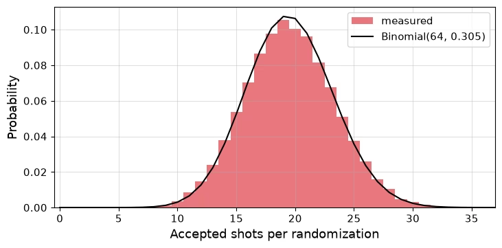
Teraz próbkujemy ponownie i uwzględniamy losowania PEC, aby złagodzić szum, którego nie wykrywają kontrole symetrii. Te próbki zostaną użyte do obliczenia wartości oczekiwanych przy użyciu wykrywania błędów w połączeniu z PEC. Poniżej wykreślamy liczbę zaakceptowanych strzałów na losowanie PEC w porównaniu z rozkładem dwumianowym przy średnim współczynniku akceptacji. Widzimy, że akceptacja jest nieskorelowana z próbkowaną instancją obwodu, ponieważ QED+PEC wstrzykuje jedynie niewykrywalne operatory Pauliego, które komutują z pomiarami każdego kubitu mediatorowego.

def launch(session, template, samplex, samplex_args, n_rand, shots_per_rand):
    """Sample `n_rand` randomizations of `template` on `session` in <=100k-randomization jobs; returns the jobs."""
    jobs = []
    for start in range(0, n_rand, 100_000):
        program = QuantumProgram(shots=shots_per_rand)
        program.append_samplex_item(
            template,
            samplex=samplex,
            samplex_arguments=samplex_args,
            shape=(min(100_000, n_rand - start), 1),
        )
        jobs.append(Executor(session, options=executor_options).run(program))
    return jobs

# Reduced PEC
args_post = {
    "pauli_lindblad_maps": dict(noise_maps),
    basis_key: meas_basis,
    **{f"noise_scales.{k}": -1.0 for k in local_scales},
    **{f"local_scales.{k}": v for k, v in local_scales.items()},
}
# PEC on the full noise model
args_van = {
    "pauli_lindblad_maps": dict(noise_maps),
    basis_key: meas_basis,
    **{f"noise_scales.{k}": -1.0 for k in local_scales},
}

# Run sampling jobs
jobs = launch(
    session, template_checked, samplex, args_post, N_RAND, SHOTS_PER_RAND
)
jobs_van = launch(
    session, template_checked, samplex, args_van, N_RAND, SHOTS_PER_RAND
)
outs = [j.result()[0] for j in jobs]
outs_van = [j.result()[0] for j in jobs_van]
(out_tw,) = job_tw.result()
session.close()

Zbierz próbki i zweryfikuj, że losowania PEC komutują z pomiarami na kubitach mediatorowych i nie wpływają na statystyki postselekcji.

def bitflip_mask(out, selector):
    """Per-shot True/False for job result `out`: shot passes `selector`'s non-Markovian error checks."""
    regs = {
        k: np.asarray(out[k])
        for k in out
        if not k.startswith(("measurement_flips", "pauli_signs"))
    }
    return selector.compute_mask(regs, "edge", mode="post")

def symmetry_mask(out):
    """Per-shot True/False for job result `out`: every twirl-corrected symmetry check reads 0."""
    return ~(
        np.asarray(out["check"]) ^ np.asarray(out["measurement_flips.check"])
    ).any(axis=-1)

def keep_mask(out, selector):
    """Per-shot True/False for job result `out`: shot passes both check types."""
    return symmetry_mask(out) & bitflip_mask(out, selector)

def fracs(out_list, selector):
    """Fractions of shots across the job results in `out_list` passing [no, non-Markovian error, symmetry, both] checks."""
    bf = np.concatenate([bitflip_mask(o, selector) for o in out_list])
    sy = np.concatenate([symmetry_mask(o) for o in out_list])
    return [1.0, bf.mean(), sy.mean(), (bf & sy).mean()]

mask_post = np.concatenate([keep_mask(o, selector) for o in outs])

# Collect the sampled data alongside the learned model, in the form the figure helpers expect
mit.update(
    ps_fracs=np.array(
        [
            fracs([out_tw], selector),
            fracs(outs_van, selector),
            fracs(outs, selector),
        ]
    ),
    acc_counts_post=np.squeeze(mask_post).sum(axis=-1),
    data_tw=np.asarray(out_tw["data"]),
    flips_tw=np.asarray(out_tw["measurement_flips.data"]),
    mask_tw=keep_mask(out_tw, selector),
    data_post=np.packbits(
        np.concatenate([np.asarray(o["data"]) for o in outs]), axis=-1
    ),
    flips_post=np.concatenate(
        [np.asarray(o["measurement_flips.data"]) for o in outs]
    ),
    signs_post=np.concatenate([np.asarray(o["pauli_signs"]) for o in outs]),
    mask_post=mask_post,
    data_van=np.packbits(
        np.concatenate([np.asarray(o["data"]) for o in outs_van]), axis=-1
    ),
    flips_van=np.concatenate(
        [np.asarray(o["measurement_flips.data"]) for o in outs_van]
    ),
    signs_van=np.concatenate(
        [np.asarray(o["pauli_signs"]) for o in outs_van]
    ),
    mask_van=np.concatenate([bitflip_mask(o, selector) for o in outs_van]),
)

# Plot the PEC bias check
plot_postselection(mit)

Oblicz wartości oczekiwane i porównaj strategie

Na koniec obliczamy wszystkie wartości oczekiwane za pomocą funkcji pomocniczej executor_expectation_values z qiskit-mitigation, która stosuje za nas odwrócenia pomiarów, maski postselekcji, współczynniki przeskalowania TREX oraz znaki quasi-prawdopodobieństwa.

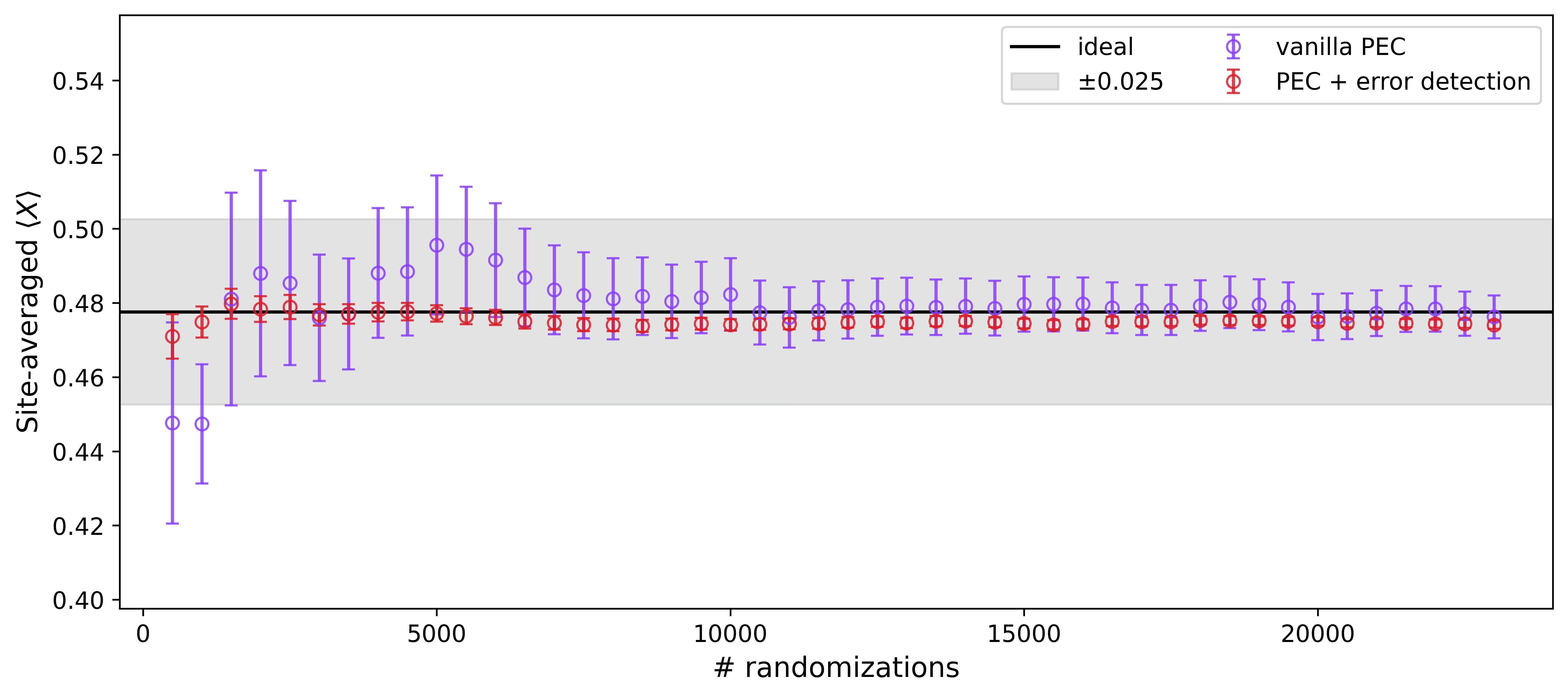
Górny wykres: Widzimy, że oba warianty PEC są zbieżne, ale QED+PEC osiąga pasmo $\pm 0.025$ przy mniejszej liczbie losowań i węższych słupkach błędów. Resztkowe obciążenie w obliczeniu QED+PEC jest poniżej 0,01 i można je przypisać pewnej kombinacji rozbieżności modelu szumu, dryfu kubitów w czasie oraz efektów niemodelowanych źródeł szumu.

Dolny wykres: Bieżący szacunek uśrednionego dla miejsc $\langle X \rangle$ w miarę gromadzenia się losowań, przy zastosowaniu identycznej liczby strzałów na losowanie dla obu wariantów PEC. PEC + wykrywanie błędów osiąga pasmo w ciągu kilku tysięcy losowań; sam PEC, ponosząc pełny narzut próbkowania, wymaga znacznie więcej losowań, aby osiągnąć zbieżność.

from qiskit.quantum_info import SparsePauliOp
from qiskit_mitigation.utils import executor_expectation_values

gamma, gamma_post = mit["gammas"]
basis_map = {Pauli("X" * n_data): [SparsePauliOp(o) for o in observables]}
rescale = dict(zip(observables, mit["trex_rescale"], strict=True))

def evs(bits, basis_map, **kwargs):
    """Per-site (means, standard errors) from boolean shot data `bits` of shape (rands, 1, shots, n_data)."""
    out = executor_expectation_values(
        bits, basis_map, None, avg_axis=(0, 1), **kwargs
    )
    return np.array([m for m, _ in out]).ravel(), np.sqrt(
        [v for _, v in out]
    ).ravel()

def unpack(mit, prefix, n_data):
    """Restore `mit[f"data_\{prefix\}"]` from packed bytes to booleans of shape (rands, 1, shots, n_data)."""
    return np.unpackbits(mit[f"data_{prefix}"], axis=-1)[..., :n_data].astype(
        bool
    )

unmit_tw, unmit_tw_err = evs(
    mit["data_tw"], basis_map, measurement_flips=mit["flips_tw"]
)
ed_tw, ed_tw_err = evs(
    mit["data_tw"],
    basis_map,
    measurement_flips=mit["flips_tw"],
    postselect_mask=mit["mask_tw"],
    rescale_factors=rescale,
)
post, post_err = evs(
    unpack(mit, "post", n_data),
    basis_map,
    measurement_flips=mit["flips_post"],
    pauli_signs=mit["signs_post"],
    postselect_mask=mit["mask_post"],
    rescale_factors=rescale,
)
pec, pec_err = evs(
    unpack(mit, "van", n_data),
    basis_map,
    measurement_flips=mit["flips_van"],
    pauli_signs=mit["signs_van"],
    postselect_mask=mit["mask_van"],
    rescale_factors=rescale,
)

# effective ED+PEC overhead measured from the data: accepted shots per signed accepted shot
signs_post = 1 - 2 * (np.squeeze(mit["signs_post"]).sum(axis=-1) % 2)
gamma_eff = (
    mit["mask_post"].sum()
    / (signs_post * np.squeeze(mit["mask_post"]).sum(axis=-1)).sum()
)

print(
    f"gamma PEC {gamma:.2f} | gamma QED+PEC {gamma_post:.2f} (model) / {gamma_eff:.2f} (data) | "
    f"QED survival {mit['mask_tw'].mean():.3f} | QED+PEC survival {mit['mask_post'].mean():.3f} | "
    f"mean QED+PEC err {post_err.mean():.4f}"
)
plot_final(
    obs_exact,
    (unmit_tw, unmit_tw_err),
    (ed_tw, ed_tw_err),
    (pec, pec_err),
    (post, post_err),
    (gamma, gamma_post),
    x_labels(layout, n_data),
    "",
)

gamma PEC 10.08 | gamma QED+PEC 2.52 (model) / 2.51 (data) | QED survival 0.304 | QED+PEC survival 0.305 | mean QED+PEC err 0.0037

plot_convergence(mit, obs_exact, n_data)