Rozpoczynanie QAOA metodą warm-start z dodatkiem Qiskit Optimization Mapper

Szacowany czas wykorzystania: 9 minut na Heron r3 (UWAGA: To tylko szacunek. Twój rzeczywisty czas wykonania może się różnić.)

Efekty nauki

• Jak odwzorować problem max-cut na kwantowe sformułowanie kwadratowej optymalizacji binarnej bez ograniczeń (QUBO) za pomocą qiskit-addon-opt-mapper

• Jak zaimplementować i uruchomić standardowe QAOA na symulatorze

• Jak zastosować WS-QAOA poprzez obliczenie relaksacji programu kwadratowego (QP) i zbudowanie obwodu warm-start

• Jak porównać zbieżność energii i jakość rozwiązania między standardowym QAOA a WS-QAOA

Wymagania wstępne

• Tutorial o QAOA

• Zaawansowany tutorial o QAOA

Kontekst

Algorytm QAOA (Quantum Approximate Optimization Algorithm) to hybrydowy algorytm kwantowo-klasyczny zaprojektowany do rozwiązywania problemów optymalizacji kombinatorycznej, takich jak max-cut i ogólne sformułowania QUBO. Podstawowe wprowadzenie do QAOA w Qiskit znajdziesz w tutorialu o QAOA; bardziej zaawansowane techniki budowania obwodów znajdziesz w zaawansowanym tutorialu o QAOA.

W standardowym QAOA:

• Stan początkowy to jednorodna superpozycja $|+\rangle^{\otimes n}$.
• Parametry wariacyjne są inicjalizowane losowo.
• Klasyczny optymalizator szuka parametrów, które minimalizują funkcję kosztu.

Jednak w przypadku praktycznych rozmiarów problemów i zaszumionego sprzętu kwantowego losowa inicjalizacja może prowadzić do wolnej zbieżności, słabych minimów lokalnych i zwiększonego kosztu optymalizacji.

QAOA z ciepłym startem (WS-QAOA) poprawia to, włączając klasyczne wnioski z optymalizacji bezpośrednio do obwodu kwantowego. Ten samouczek opiera się na metodach wprowadzonych przez Eggera, Marečka i Woernera w Warm-starting quantum optimization. Kluczowa idea polega na tym, aby:

1. Rozwiązać relaksację ciągłą oryginalnego problemu binarnego (program kwadratowy nad $[0,1]^n$ zamiast $\{0,1\}^n$).

2. Zakodować rozwiązanie zrelaksowane $c^*_i \in [0,1]$ w niestandardowym stanie początkowym, używając kątów rotacji $Y$: $\theta_i = 2\arcsin(\sqrt{c^*_i})$, tak aby kubit $i$ zaczynał w stanie, którego prawdopodobieństwo zmierzenia $|1\rangle$ wynosi $c^*_i$.

3. Zastąpić standardowy mikser $X$ niestandardowym mikserem, którego stan podstawowy jest stanem początkowym z ciepłym startem, zapewniając, że algorytm zaczyna blisko rozwiązania klasycznego i może eksplorować sąsiedztwo.

Parametr regularyzacji $\varepsilon \in [0, 0.5]$ obcina $c^*_i$ z dala od 0 i 1, aby uniknąć problemów z osiągalnością; kubity zainicjalizowane w $|0\rangle$ lub $|1\rangle$ nie mogą zostać przesunięte przez hamiltonian kosztu. Przy $\varepsilon = 0.5$ WS-QAOA redukuje się dokładnie do standardowego QAOA.

Modelowanie problemu wykorzystuje pakiet qiskit-addon-opt-mapper, którego klasa aplikacji Maxcut buduje QUBO bezpośrednio z grafu, a jego konwertery i translatory mapują wynikowy problem na hamiltoniany kwantowe.

Wymagania

Zanim rozpoczniesz ten samouczek, upewnij się, że masz zainstalowane następujące elementy:

• Qiskit SDK w wersji 2.0 lub nowszej, ze wsparciem wizualizacji

• Qiskit Runtime w wersji 0.43 lub nowszej (pip install qiskit-ibm-runtime)

• Dodatek Qiskit Optimization Mapper (pip install qiskit-addon-opt-mapper)

• SciPy (pip install scipy)

• NetworkX (pip install networkx)

Konfiguracja

Zaimportuj wszystkie wymagane biblioteki i zdefiniuj funkcje pomocnicze używane w tym samouczku.

# Added by doQumentation — required packages for this notebook
!pip install -q matplotlib networkx numpy qiskit qiskit-addon-opt-mapper qiskit-ibm-runtime scipy

import numpy as np
import matplotlib.pyplot as plt
import networkx as nx
from scipy.optimize import minimize

from qiskit.circuit import QuantumCircuit, ParameterVector
from qiskit.circuit.library import qaoa_ansatz
from qiskit.quantum_info import Statevector
from qiskit.primitives import StatevectorEstimator, StatevectorSampler
from qiskit.transpiler.preset_passmanagers import generate_preset_pass_manager
from qiskit_ibm_runtime import (
    QiskitRuntimeService,
    Session,
    EstimatorOptions,
    EstimatorV2 as Estimator,
    SamplerV2 as Sampler,
)

from qiskit_addon_opt_mapper.applications import Maxcut
from qiskit_addon_opt_mapper.converters import OptimizationProblemToQubo
from qiskit_addon_opt_mapper.translators import to_ising

Przykład symulatora na małą skalę

Jako przykład przewodni używamy małego problemu max-cut na ważonym grafie. Max-cut zadaje pytanie: mając graf $G=(V,E)$ z wagami krawędzi $w_{ij}$, znajdź podział wierzchołków na dwa zbiory $S$ i $\bar{S}$, który maksymalizuje całkowitą wagę krawędzi przecinających podział.

Jako problem minimalizacji QUBO, max-cut można zapisać jako: $\min_{x \in \{0,1\}^n} -\sum_{(i,j) \in E} w_{ij}(x_i + x_j - 2x_i x_j)$

Pracujemy z grafem czterowęzłowym dla zapewnienia sterowalności na symulatorze.

Krok 1: Mapowanie danych klasycznych na problem kwantowy

Definiujemy problem max-cut, używając klasy aplikacji Maxcut z qiskit-addon-opt-mapper, która buduje sformułowanie QUBO bezpośrednio z grafu. Następnie konwertujemy go do QUBO i tłumaczymy na hamiltonian Isinga (SparsePauliOp) odpowiedni dla QAOA. Rozwiązujemy również relaksację ciągłą QUBO — zastępując ograniczenie binarne $x_i \in \{0,1\}$ przez $x_i \in [0,1]$ — aby uzyskać punkt początkowy ciepłego startu $c^*$.

# Define a 4-node weighted graph for the max-cut problem
n_nodes = 4
edges = [(0, 1, 1.0), (0, 2, 1.0), (1, 2, 1.0), (1, 3, 1.0), (2, 3, 1.0)]

G = nx.Graph()
G.add_nodes_from(range(n_nodes))
G.add_weighted_edges_from(edges)

pos = nx.spring_layout(G, seed=42)
edge_labels = {(u, v): d["weight"] for u, v, d in G.edges(data=True)}

fig, ax = plt.subplots(figsize=(4, 3))
nx.draw(G, pos, with_labels=True, node_color="lightblue", ax=ax)
nx.draw_networkx_edge_labels(G, pos, edge_labels=edge_labels, ax=ax)
ax.set_title("Max-Cut graph")
plt.tight_layout()
plt.show()

Graf ma pięć krawędzi. Optymalny max-cut dzieli węzły na $S = \{0, 3\}$ i $\bar{S} = \{1, 2\}$ (lub dopełnienie), przecinając cztery z pięciu krawędzi, co daje wartość cięcia równą 4.

# Build the max-cut problem directly from the NetworkX graph using the
# Maxcut application class. Internally it constructs the QUBO
#   minimize  -sum_{(i,j) in E} w_ij * (x_i + x_j - 2*x_i*x_j)
# (each edge contributes -w to the linear terms and +2w to the quadratic
# term), so we get the same OptimizationProblem without the boilerplate.
maxcut = Maxcut(G)
prob = maxcut.to_optimization_problem()
print(prob.prettyprint())

Problem name: Max-cut

Maximize
  -2*x_0*x_1 - 2*x_0*x_2 - 2*x_1*x_2 - 2*x_1*x_3 - 2*x_2*x_3 + 2*x_0 + 3*x_1
  + 3*x_2 + 2*x_3

Subject to
  No constraints

  Binary variables (4)
    x_0 x_1 x_2 x_3

Klasa Maxcut opakowuje konstrukcję QUBO, dzięki czemu nie musimy ręcznie rozwijać funkcji celu max-cut. Wypisany cel pokazuje liniowy współczynnik każdej zmiennej (jak bardzo indywidualnie przyczynia się ona do cięcia) oraz kwadratowy współczynnik każdego wyrazu krzyżowego (kara za umieszczenie dwóch sąsiadujących węzłów po tej samej stronie). Bazowy OptimizationProblem zwracany przez to_optimization_problem() obsługuje zmienne binarne, całkowitoliczbowe, ciągłe i spinowe i jest tym samym obiektem, którego oczekują konwertery i translatory używane w następnym kroku.

# Convert the OptimizationProblem to a QUBO, then translate to an Ising Hamiltonian
#
# The substitution x_i = (1 - z_i)/2  maps binary variables to spin operators,
# yielding a Hamiltonian H_C = sum_i h_i Z_i + sum_{i<j} J_ij Z_i Z_j + constant.
# QAOA minimizes <H_C> to find the ground state, which encodes the optimal cut.
converter = OptimizationProblemToQubo()
qubo = converter.convert(prob)

cost_operator, offset = to_ising(qubo)
n_qubits = cost_operator.num_qubits

print(f"Cost Hamiltonian H_C ({n_qubits} qubits):")
print(cost_operator)
print(f"\nOffset (constant shift): {offset}")
print("  QUBO value = Ising energy + offset")

Cost Hamiltonian H_C (4 qubits):
SparsePauliOp(['IIZZ', 'IZIZ', 'IZZI', 'ZIZI', 'ZZII'],
              coeffs=[0.5+0.j, 0.5+0.j, 0.5+0.j, 0.5+0.j, 0.5+0.j])

Offset (constant shift): -2.5
  QUBO value = Ising energy + offset

Translator to_ising zwraca SparsePauliOp reprezentujący $H_C$ oraz skalarny offset taki, że $\text{QUBO value} = \langle H_C \rangle + \text{offset}$. Dla tego problemu max-cut ze wszystkimi jednostkowymi wagami $h_i = 0$ dla wszystkich kubitów (graf jest symetryczny w wyrazach liniowych po podstawieniu $x_i \to z_i$), a każda krawędź wnosi sprzężenie $Z_i Z_j$ o sile $+0.5$. Minimalna wartość własna $H_C$ odpowiada maksymalnemu cięciu.

# Solve the continuous (QP) relaxation to obtain the warm-start point c*
#
# The QP relaxation replaces the binary constraint x_i in {0,1} with x_i in [0,1]
# and minimizes the same quadratic objective. Its solution c*_i gives the
# probability that variable i should be 1 according to the classical relaxation.
#
# The max-cut QUBO has a non-convex quadratic matrix (negative eigenvalues),
# so the relaxed problem has multiple local minima. A naive single start from
# [0.5,...,0.5] converges to the symmetric saddle point c* = [0.5,...,0.5],
# which carries no useful structural information about the problem.
# Multi-start optimization is used to reliably find the global minimum.
Q = qubo.objective.quadratic.to_array(symmetric=True)
mu = qubo.objective.linear.to_array()

def qp_objective(x_cont):
    """Continuous relaxation of the QUBO objective."""
    return x_cont @ Q @ x_cont + mu @ x_cont + qubo.objective.constant

bounds = [(0.0, 1.0)] * n_qubits

rng = np.random.default_rng(42)
best_val = np.inf
c_star = None
for _ in range(200):
    x0 = rng.uniform(0.0, 1.0, n_qubits)
    result = minimize(qp_objective, x0, method="L-BFGS-B", bounds=bounds)
    if result.fun < best_val:
        best_val = result.fun
        c_star = result.x

print(f"QP relaxation solution c* = {np.round(c_star, 4)}")
print(f"QP objective value        = {best_val:.4f}")

QP relaxation solution c* = [1. 0. 0. 1.]
QP objective value        = -4.0000

Solver z wieloma startami znajduje $c^* = [1, 0, 0, 1]$ (lub jego dopełnienie $[0, 1, 1, 0]$), co jest rzeczywistym optymalnym rozwiązaniem binarnym. Dla tego problemu relaksacja QP jest ścisła, minimum ciągłe pokrywa się z optimum całkowitoliczbowym, co oznacza, że relaksacja od razu identyfikuje najlepsze cięcie. Po regularyzacji z $\varepsilon = 0.25$ w kroku 2 to rozwiązanie zostanie zakodowane w stanie początkowym ciepłego startu.

Krok 2: Optymalizacja problemu pod kątem wykonania na sprzęcie kwantowym

Budujemy dwa obwody QAOA i przygotowujemy kąty ciepłego startu na podstawie rozwiązania QP.

Standardowe QAOA wykorzystuje jednorodną superpozycję $|+\rangle^{\otimes n}$ jako stan początkowy oraz standardowy mikser $X$: $H_M = -\sum_i X_i$, zaimplementowany jako $\prod_i R_X(-2\beta)$ na warstwę.

QAOA z ciepłym startem (WS-QAOA) z [1] wprowadza dwie strukturalne zmiany dla każdego kubitu $i$:

• Stan początkowy: $R_Y(\theta_i)|0\rangle$ z $\theta_i = 2\arcsin(\sqrt{c^*_i})$, tak że prawdopodobieństwo zmierzenia $|1\rangle$ jest równe $c^*_i$.
• Niestandardowy mikser: $R_Y(\theta_i)\, R_Z(-2\beta)\, R_Y(-\theta_i)$, którego stanem podstawowym jest $R_Y(\theta_i)|0\rangle$. Oznacza to, że WS-QAOA zaczyna w stanie podstawowym swojego własnego miksera, tej samej właściwości, którą standardowe QAOA spełnia dla $|+\rangle$ i miksera $X$.

Uwaga dotycząca warstw: przy p=1 (pojedyncza warstwa QAOA) standardowe QAOA jest analitycznie ograniczone do ~49% optymalnej energii na grafach zawierających trójkąty (ten graf zawiera trójkąt 0-1-2). Ciepły start omija to ograniczenie, kodując wcześniejszą wiedzę o rozwiązaniu bezpośrednio w stanie początkowym.

# Number of QAOA layers (each layer = one cost unitary + one mixer unitary)
p = 1

# Regularization: clip c* to [epsilon, 1-epsilon] so no qubit is initialized
# in |0> or |1>, which would freeze it under the cost Hamiltonian.
epsilon = 0.25

c_clipped = np.clip(c_star, epsilon, 1 - epsilon)
thetas = 2 * np.arcsin(np.sqrt(c_clipped))

print(f"Continuous relaxation c*  = {np.round(c_star, 4)}")
print(f"After regularization      = {np.round(c_clipped, 4)}")
print(f"Warm-start angles theta   = {np.round(thetas, 4)} radians")
print()
print("Angle interpretation:")
print("  theta = 0      <->  c* = 0   (qubit points toward |0>)")
print(
    "  theta = pi/2   <->  c* = 0.5 (qubit in equal superposition, like |+>)"
)
print("  theta = pi     <->  c* = 1   (qubit points toward |1>)")

Continuous relaxation c*  = [1. 0. 0. 1.]
After regularization      = [0.75 0.25 0.25 0.75]
Warm-start angles theta   = [2.0944 1.0472 1.0472 2.0944] radians

Angle interpretation:
  theta = 0      <->  c* = 0   (qubit points toward |0>)
  theta = pi/2   <->  c* = 0.5 (qubit in equal superposition, like |+>)
  theta = pi     <->  c* = 1   (qubit points toward |1>)

Po obcięciu $c^* = 1$ staje się $1 - \varepsilon = 0.75$, a $c^* = 0$ staje się $\varepsilon = 0.25$. Wynikowe kąty $\theta \approx [2.09, 1.05, 1.05, 2.09]$ radianów obracają kubity 0 i 3 silnie w stronę $|1\rangle$, a kubity 1 i 2 w stronę $|0\rangle$, bezpośrednio kodując strukturę optymalnego cięcia w stanie początkowym kwantowym.

def apply_cost_unitary(qc, cost_op, gamma):
    """Apply exp(-i * gamma * H_C) to the circuit.

    Each Pauli term in H_C contributes a rotation gate:
      - Single-Z term h_i * Z_i  ->  RZ(2 * gamma * h_i) on qubit i
      - Two-Z term J_ij * Z_i Z_j  ->  CNOT, RZ(2 * gamma * J_ij), CNOT
    """
    for pauli_term, coeff in zip(cost_op.paulis, cost_op.coeffs):
        indices = [
            j for j, q in enumerate(pauli_term.to_label()[::-1]) if q == "Z"
        ]
        if len(indices) == 1:
            qc.rz(2 * gamma * coeff.real, indices[0])
        elif len(indices) == 2:
            qc.cx(indices[0], indices[1])
            qc.rz(2 * gamma * coeff.real, indices[1])
            qc.cx(indices[0], indices[1])

def build_ws_qaoa(cost_op, n_layers, n_qubits, thetas):
    """WS-QAOA: warm-start initial state + custom per-qubit mixer.

    Per Egger et al. (2021) Eq. (1)-(2):
      Initial state per qubit i:  R_Y(theta_i) |0>
      Mixer gate per qubit i:     R_Y(theta_i) R_Z(-2*beta) R_Y(-theta_i)
    """
    gammas = ParameterVector("γ", n_layers)
    betas = ParameterVector("β", n_layers)
    qc = QuantumCircuit(n_qubits)
    for i, theta in enumerate(thetas):
        qc.ry(theta, i)  # warm-start initial state
    for k in range(n_layers):
        apply_cost_unitary(qc, cost_op, gammas[k])
        for i, theta in enumerate(thetas):
            qc.ry(theta, i)
            qc.rz(-2 * betas[k], i)
            qc.ry(-theta, i)
    return qc, gammas, betas

# Standard QAOA via the Qiskit built-in helper:
# qaoa_ansatz prepares |+>^n, then alternates exp(-i*gamma*H_C) with the
# default X-mixer for `reps` layers. The returned circuit exposes the
# variational parameters via std_qc.parameters.
std_qc = qaoa_ansatz(cost_operator, reps=p)

# WS-QAOA: keep the custom builder. The per-qubit mixer
# R_Y(theta_i) R_Z(-2*beta) R_Y(-theta_i) is implemented as an explicit gate
# sequence rather than as a SparsePauliOp, so we construct the circuit
# directly to stay close to the Egger et al. (2021) formulation.
ws_qc, ws_gammas, ws_betas = build_ws_qaoa(cost_operator, p, n_qubits, thetas)

Dla standardowego ansatzu delegujemy do qaoa_ansatz, który konstruuje $|+\rangle^{\otimes n}$, stosuje unitarność kosztu i stosuje domyślny mikser $X$ dla każdej z reps warstw. Dla WS-QAOA zachowujemy jawnego pomocnika build_ws_qaoa, ponieważ mikser dla każdego kubitu $R_Y(\theta)\,R_Z(-2\beta)\,R_Y(-\theta)$ jest wyrażony jako sekwencja bramek, a nie jako suma Paulich. Pomocnik apply_cost_unitary czyta bezpośrednio z hamiltonianu SparsePauliOp, więc obsługuje dowolny problem QUBO bez ręcznej konstrukcji obwodu.

print("Standard QAOA circuit (p=1):")
std_qc.draw("mpl", fold=-1)

Standard QAOA circuit (p=1):

print("\nWS-QAOA circuit (p=1):")
ws_qc.draw("mpl", fold=-1)

WS-QAOA circuit (p=1):

Oba obwody mają tę samą strukturę: warstwę przygotowania stanu początkowego, a następnie $p$ na przemian warstw unitarności kosztu i unitarności miksera. W obwodzie WS-QAOA początkowe bramki $R_Y$ kodują $c^*$, a mikser zastępuje każdą bramkę $R_X$ sprzężoną trójką $R_Y$–$R_Z$–$R_Y$. Różnica głębokości obwodu między tymi dwoma podejściami rośnie liniowo wraz z $p$, ale pozostaje możliwa do opanowania przy niskiej głębokości.

Krok 3: Wykonanie z użyciem prymitywów Qiskit

Używamy StatevectorEstimator do dokładnej, bezszumowej symulacji. Funkcja minimize z SciPy z optymalizatorem COBYLA napędza pętlę wariacyjną, wywołując estymator przy każdej iteracji, aby ocenić $\langle H_C \rangle$ dla danego zestawu parametrów $(\gamma, \beta)$.

Oba algorytmy używają różnych parametrów początkowych, które odzwierciedlają to, co każdy z nich wie przed optymalizacją:

• Standardowe QAOA: Losowa inicjalizacja w $[0, \pi]$ — odpowiednia, ponieważ nie są dostępne żadne informacje strukturalne.
• WS-QAOA: $\gamma = 0$, $\beta = \pi/4$ — przy $\gamma=0$ unitarność kosztu jest tożsamością, więc pierwsza sama w sobie ewaluacja obwodu próbkuje bezpośrednio ze stanu początkowego ciepłego startu. Daje to COBYLA silny sygnał startowy zgodny z rozwiązaniem klasycznym.

estimator = StatevectorEstimator()

def make_cost_fn(circuit, param_order, cost_op, estimator, history):
    """Return a scalar cost function compatible with scipy.optimize.minimize."""

    def cost_fn(params):
        bound = circuit.assign_parameters(dict(zip(param_order, params)))
        job = estimator.run([(bound, cost_op)])
        energy = job.result()[0].data.evs.real
        history.append(energy)
        return energy

    return cost_fn

# Standard QAOA: random initialization
np.random.seed(42)
std_param_order = list(std_qc.parameters)
std_params0 = np.random.uniform(0, np.pi, len(std_param_order))
std_history = []

std_result = minimize(
    make_cost_fn(
        std_qc, std_param_order, cost_operator, estimator, std_history
    ),
    std_params0,
    method="COBYLA",
    options={"maxiter": 300, "rhobeg": 0.5},
)
print(f"Standard QAOA optimal energy : {std_result.fun:.4f}")
print(f"  optimal params: {std_result.x.round(4)}")
print(f"  optimizer calls: {len(std_history)}")

# WS-QAOA: informed initialization
ws_params0 = np.concatenate([np.zeros(p), np.full(p, np.pi / 4)])
ws_history = []
ws_param_order = list(ws_gammas) + list(ws_betas)

ws_result = minimize(
    make_cost_fn(ws_qc, ws_param_order, cost_operator, estimator, ws_history),
    ws_params0,
    method="COBYLA",
    options={"maxiter": 300, "rhobeg": 0.5},
)
print(f"\nWS-QAOA optimal energy       : {ws_result.fun:.4f}")
print(
    f"  optimal params: gamma={ws_result.x[:p].round(4)}, beta={ws_result.x[p:].round(4)}"
)
print(f"  optimizer calls: {len(ws_history)}")

Standard QAOA optimal energy : -0.5859
  optimal params: [0.6803 2.0533]
  optimizer calls: 47

WS-QAOA optimal energy       : -1.5000
  optimal params: gamma=[-0.0001], beta=[1.5708]
  optimizer calls: 42

Świadomy punkt startowy WS-QAOA oznacza, że COBYLA zaczyna od znaczącej wartości energii blisko rozwiązania ciepłego startu, podczas gdy standardowe QAOA zaczyna z zasadniczo losowego punktu na krajobrazie energii. Ta różnica w jakości startu jest głównym czynnikiem napędzającym lukę w zbieżności widoczną w kroku 4.

# Compute the exact optimal energy by brute-force over all 2^n bitstrings
all_energies = [
    Statevector.from_label(format(k, f"0{n_qubits}b"))
    .expectation_value(cost_operator)
    .real
    for k in range(2**n_qubits)
]
optimal_energy = min(all_energies)

print(f"Exact optimal energy         : {optimal_energy:.4f}")
print(f"Standard QAOA approx. ratio  : {std_result.fun / optimal_energy:.4f}")
print(f"WS-QAOA approx. ratio        : {ws_result.fun / optimal_energy:.4f}")

Exact optimal energy         : -1.5000
Standard QAOA approx. ratio  : 0.3906
WS-QAOA approx. ratio        : 1.0000

Współczynnik aproksymacji jest zdefiniowany jako $\langle H_C \rangle_{\text{QAOA}} / E_{\text{opt}}$. Dla problemów minimalizacji, w których $E_{\text{opt}} < 0$, współczynnik bliższy 1 oznacza, że algorytm znalazł niższą energię (lepsze rozwiązanie). Wyczerpujące przeszukiwanie wszystkich $2^n$ stanów bazowych jest wykonalne tylko dla małych $n$ i służy jako punkt odniesienia dla prawdziwej wartości.

Krok 4: Postprzetwarzanie i zwrócenie wyniku w pożądanym formacie klasycznym

Wizualizujemy zbieżność, próbkujemy zoptymalizowane obwody w poszukiwaniu rozwiązań w postaci ciągów bitowych, dekodujemy te ciągi bitowe z powrotem na podziały max-cut i podsumowujemy końcowe wyniki.

fig, ax = plt.subplots(figsize=(7, 4))
ax.plot(std_history, label="Standard QAOA", alpha=0.85)
ax.plot(ws_history, label="WS-QAOA", alpha=0.85)
ax.axhline(
    optimal_energy,
    color="k",
    linestyle="--",
    label=f"Exact optimal ({optimal_energy:.2f})",
)
ax.set_xlabel("Optimizer call")
ax.set_ylabel(r"$\langle H_C \rangle$")
ax.set_title("Convergence: Standard QAOA vs. WS-QAOA")
ax.legend()
plt.tight_layout()
plt.show()

Wykres zbieżności pokazuje energię $\langle H_C \rangle$ przy każdej ewaluacji funkcji COBYLA. Standardowe QAOA przy $p=1$ jest ograniczone do ~49% optymalnej energii na tym grafie (teoretyczne maksimum dla QAOA z $p=1$ na grafach z trójkątami), stabilizując się w okolicach $-0.74$. WS-QAOA, zainicjalizowane blisko optymalnego rozwiązania, szybko zbiega do wartości bliskiej $-1.50$ (dokładne optimum) przy znacznie mniejszej liczbie iteracji. Pokazuje to kluczową zaletę ciepłego startu: przy tej samej głębokości obwodu osiąga on znacznie lepsze rozwiązanie.

# Sample the optimized circuits to recover the most probable bitstring solutions
sampler = StatevectorSampler()
shots = 1024

def get_best_bitstring(circuit, param_order, optimal_params, sampler, shots):
    bound = circuit.assign_parameters(dict(zip(param_order, optimal_params)))
    bound.measure_all()
    job = sampler.run([bound], shots=shots)
    counts = job.result()[0].data.meas.get_counts()
    return max(counts, key=counts.get), counts

def evaluate_cut(bitstring, G):
    """Compute the Max-Cut value for a bitstring node assignment."""
    x = [int(b) for b in bitstring]
    cut_val = sum(
        w for u, v, w in G.edges.data("weight", default=1) if x[u] != x[v]
    )
    set0 = [i for i, b in enumerate(bitstring) if b == "0"]
    set1 = [i for i, b in enumerate(bitstring) if b == "1"]
    return cut_val, set0, set1

# Qiskit bitstring ordering: rightmost character = qubit 0
def decode_bitstring(bs):
    return bs[::-1]

std_best, std_counts = get_best_bitstring(
    std_qc, std_param_order, std_result.x, sampler, shots
)
ws_best, ws_counts = get_best_bitstring(
    ws_qc, ws_param_order, ws_result.x, sampler, shots
)

std_cut, std_s0, std_s1 = evaluate_cut(decode_bitstring(std_best), G)
ws_cut, ws_s0, ws_s1 = evaluate_cut(decode_bitstring(ws_best), G)

print(f"Standard QAOA most-probable bitstring : {std_best}")
print(f"  Partition: S={std_s0}, S̄={std_s1}  |  cut value = {std_cut}")
print()
print(f"WS-QAOA most-probable bitstring       : {ws_best}")
print(f"  Partition: S={ws_s0}, S̄={ws_s1}  |  cut value = {ws_cut}")

Standard QAOA most-probable bitstring : 0110
  Partition: S=[0, 3], S̄=[1, 2]  |  cut value = 4.0

WS-QAOA most-probable bitstring       : 0110
  Partition: S=[0, 3], S̄=[1, 2]  |  cut value = 4.0

Ciągi bitowe z Sampler są zwracane z kubitem 0 na skrajnie prawej pozycji, więc odwrócenie ciągu mapuje indeks $i$ na zmienną $x_i$. Wartość cięcia to całkowita waga krawędzi przecinających podział, co jest tym, co problem max-cut ma na celu zmaksymalizować. Wartość cięcia równa 4 wykorzystuje cztery z pięciu dostępnych krawędzi, co jest teoretycznym maksimum dla tego grafu.

# Visualize the WS-QAOA solution on the graph
fig, axes = plt.subplots(1, 2, figsize=(8, 3))

for ax, s0, s1, cut, title in [
    (axes[0], std_s0, std_s1, std_cut, f"Standard QAOA (cut = {std_cut})"),
    (axes[1], ws_s0, ws_s1, ws_cut, f"WS-QAOA (cut = {ws_cut})"),
]:
    colors = ["skyblue" if i in s0 else "salmon" for i in G.nodes()]
    nx.draw(G, pos, with_labels=True, node_color=colors, ax=ax)
    nx.draw_networkx_edge_labels(G, pos, edge_labels=edge_labels, ax=ax)
    ax.set_title(title)

plt.tight_layout()
plt.show()

# Summary
# to_ising offset: QUBO value = Ising energy + offset, so Max-Cut value = -(Ising energy + offset)
optimal_cut = -(optimal_energy + offset)
print("=== Summary ===")
print(
    f"{'Method':<20} {'Ising energy':>14} {'Cut value':>12} {'Approx. ratio':>15}"
)
print("-" * 65)
print(
    f"{'Standard QAOA':<20} {std_result.fun:>14.4f} {std_cut:>12} {std_result.fun/optimal_energy:>15.4f}"
)
print(
    f"{'WS-QAOA':<20} {ws_result.fun:>14.4f} {ws_cut:>12} {ws_result.fun/optimal_energy:>15.4f}"
)
print(
    f"{'Exact optimal':<20} {optimal_energy:>14.4f} {optimal_cut:>12.0f} {'1.0000':>15}"
)

=== Summary ===
Method                 Ising energy    Cut value   Approx. ratio
-----------------------------------------------------------------
Standard QAOA               -0.5859          4.0          0.3906
WS-QAOA                     -1.5000          4.0          1.0000
Exact optimal               -1.5000            4          1.0000

Wizualizacja grafu koloruje każdy węzeł według przypisania do podziału (niebieski = $S$, pomarańczowy = $\bar{S}$). Krawędzie przecinające podział (łączące węzły o różnych kolorach) to te, które są liczone do cięcia.

Obie metody znajdują ciąg bitowy o wartości cięcia 4, ale z bardzo różnych powodów. Ważne jest, aby zauważyć, że wykres zbieżności i próbkowany ciąg bitowy mierzą dwie różne rzeczy:

• Wykres zbieżności śledzi średnią energię $\langle H_C \rangle$ pełnego stanu kwantowego, ważoną średnią po wszystkich ciągach bitowych w superpozycji. Standardowe QAOA zbiega do ~$-0.62$, znacznie powyżej optymalnego $-1.50$, co oznacza, że jego stan kwantowy jest rozproszony na wielu suboptymalnych ciągach bitowych i tylko okazjonalnie zawiera poprawną odpowiedź.

• Próbkowany ciąg bitowy to pojedyncze losowanie z tego stanu. Standardowe QAOA miało tutaj szczęście; optymalny podział okazał się najczęściej próbkowanym wynikiem nawet z rozproszonego stanu. W przypadku trudniejszych problemów, bardziej zaszumionego sprzętu lub większej liczby konkurujących rozwiązań kandydujących to szczęście się kończy.

WS-QAOA, w przeciwieństwie do tego, zbiega swoją średnią energię aż do $-1.50$, co oznacza, że jego stan kwantowy jest skoncentrowany na optymalnych ciągach bitowych. Niemal każdy strzał zwraca poprawną odpowiedź, więc rozwiązanie jest znajdowane niezawodnie, a nie przez przypadek.

Praktyczna konsekwencja: na tym małym, bezszumowym symulatorze różnica może wydawać się niewielka, ale przy większych rozmiarach problemów lub na prawdziwym sprzęcie stan o średniej energii bliskiej optimum jest znacznie bardziej odporny niż taki, który tylko okazjonalnie próbkuje poprawną odpowiedź z rozproszonego rozkładu.

# Compare the full probability distribution over cut values for both
# algorithms. The most-probable bitstring above only reveals the mode;
# this histogram exposes how much of the quantum state's probability mass
# lands on the optimal cut versus on suboptimal partitions.
def cut_value_distribution(counts, G, shots):
    dist = {}
    for bs, c in counts.items():
        cut, _, _ = evaluate_cut(decode_bitstring(bs), G)
        dist[cut] = dist.get(cut, 0.0) + c / shots
    return dist

std_cut_dist = cut_value_distribution(std_counts, G, shots)
ws_cut_dist = cut_value_distribution(ws_counts, G, shots)

cut_values = sorted(set(std_cut_dist) | set(ws_cut_dist))
std_probs = [std_cut_dist.get(c, 0.0) for c in cut_values]
ws_probs = [ws_cut_dist.get(c, 0.0) for c in cut_values]

fig, ax = plt.subplots(figsize=(7, 4))
x = np.arange(len(cut_values))
width = 0.4
ax.bar(
    x - width / 2, std_probs, width, label="Standard QAOA", color="steelblue"
)
ax.bar(x + width / 2, ws_probs, width, label="WS-QAOA", color="salmon")
ax.axvline(
    cut_values.index(optimal_cut),
    color="k",
    linestyle="--",
    alpha=0.4,
    label=f"Optimal cut = {optimal_cut:g}",
)
ax.set_xticks(x)
ax.set_xticklabels([f"{c:g}" for c in cut_values])
ax.set_xlabel("Cut value")
ax.set_ylabel("Probability")
ax.set_title(f"Probability of measuring each cut value ({shots} shots)")
ax.legend()
plt.tight_layout()
plt.show()

print(
    f"P(cut = {optimal_cut:g}) | Standard QAOA = "
    f"{std_cut_dist.get(optimal_cut, 0):.4f}  "
    f"WS-QAOA = {ws_cut_dist.get(optimal_cut, 0):.4f}"
)

P(cut = 4) | Standard QAOA = 0.4639  WS-QAOA = 1.0000

Ten histogram kwantyfikuje to, co wykres zbieżności tylko sugerował. Prawdopodobieństwo standardowego QAOA jest rozproszone pomiędzy wieloma suboptymalnymi wartościami cięcia, więc szansa na wylosowanie optymalnego cięcia o wartości cztery w pojedynczym strzale to tylko ułamek całkowitej masy. WS-QAOA koncentruje niemal całe swoje prawdopodobieństwo na optymalnym cięciu, więc niemal każdy strzał zwraca poprawną odpowiedź. To praktyczna sygnatura stanu, którego średnia energia zbiegła do energii stanu podstawowego, w przeciwieństwie do stanu, który po prostu przypadkowo zawierał stan podstawowy w szerokiej superpozycji.

Przykład sprzętu na dużą skalę

Kroki 1-4 skompresowane w jeden blok kodu

# Selecting a backend using real hardware
service = QiskitRuntimeService()
backend = service.least_busy(
    operational=True, simulator=False, min_num_qubits=127
)
print(f"Using backend: {backend.name}")

Using backend: ibm_boston

# ── Step 1a: Build the 40-node Max-Cut problem ─────────────────────────────
# A 3-regular graph (every node has exactly 3 neighbors) is a standard QAOA
N_LARGE = 40
G_large = nx.random_regular_graph(d=3, n=N_LARGE, seed=0)
edges_large = list(G_large.edges())
print(f"Graph: {N_LARGE} nodes, {len(edges_large)} edges (3-regular)")

# Visualize the graph so it is clear what problem we are solving before any
# quantum work. Nodes in a circular layout; each edge contributes +1 to the
# cut value when its endpoints land in different partitions.
pos_large = nx.circular_layout(G_large)
fig, ax = plt.subplots(figsize=(6, 6))
nx.draw(
    G_large,
    pos_large,
    with_labels=True,
    node_color="lightblue",
    node_size=400,
    font_size=7,
    ax=ax,
)
ax.set_title(f"40-node 3-regular Max-Cut graph ({len(edges_large)} edges)")
plt.tight_layout()
plt.show()

# Same Maxcut → OptimizationProblem → QUBO → Ising pipeline as the small example,
# applied to the 40-node graph.
prob_large = Maxcut(G_large).to_optimization_problem()
converter_large = OptimizationProblemToQubo()
qubo_large = converter_large.convert(prob_large)
cost_op_large, offset_large = to_ising(qubo_large)
n_qubits_large = cost_op_large.num_qubits
print(
    f"Cost operator: {n_qubits_large} qubits, {len(cost_op_large)} Pauli terms"
)

# ── Step 1b: QP relaxation (multi-start L-BFGS-B) ─────────────────────────
# Same multi-start approach as the small example. At 40 qubits the relaxed
# landscape has many more local minima, so 200 random starts are essential
# to find a low-energy warm-start point.
Q_large = qubo_large.objective.quadratic.to_array(symmetric=True)
mu_large = qubo_large.objective.linear.to_array()

def qp_obj_large(x):
    return x @ Q_large @ x + mu_large @ x + qubo_large.objective.constant

bounds_large = [(0.0, 1.0)] * n_qubits_large
rng_qp = np.random.default_rng(42)
best_val_large, c_star_large = np.inf, None

for _ in range(200):
    x0 = rng_qp.uniform(0.0, 1.0, n_qubits_large)
    res = minimize(qp_obj_large, x0, method="L-BFGS-B", bounds=bounds_large)
    if res.fun < best_val_large:
        best_val_large, c_star_large = res.fun, res.x

# Regularize and convert to rotation angles (same formula as small example)
epsilon_large = 0.25
c_clipped_large = np.clip(c_star_large, epsilon_large, 1 - epsilon_large)
thetas_large = 2 * np.arcsin(np.sqrt(c_clipped_large))
print(
    f"c* range: [{c_star_large.min():.3f}, {c_star_large.max():.3f}]  "
    f"theta range: [{thetas_large.min():.3f}, {thetas_large.max():.3f}] rad"
)

# Plot the distribution of c* values to see how much structure the relaxation
# extracted. Values near 0/1 mean confident assignments; values near 0.5 mean
# the classical solver was uncertain and quantum exploration is most needed there.
fig, ax = plt.subplots(figsize=(6, 3))
ax.hist(c_star_large, bins=20, color="steelblue", edgecolor="white")
ax.axvline(0.5, color="k", linestyle="--", label="Uniform prior (std QAOA)")
ax.set_xlabel(r"$c^*_i$")
ax.set_ylabel("Count")
ax.set_title(r"Distribution of warm-start values $c^*_i$ (40-node graph)")
ax.legend()
plt.tight_layout()
plt.show()

# ── Step 1c: Build WS-QAOA circuit ─────────────────────────────────────────
# Reuse build_ws_qaoa from the small-scale section unchanged; the helper
# scales automatically with n_qubits and the cost operator size.
p_large = 1
ws_qc_large, ws_gammas_large, ws_betas_large = build_ws_qaoa(
    cost_op_large, p_large, n_qubits_large, thetas_large
)
ws_qc_large.measure_all()

# ── Step 2: Transpile to hardware-native gates ──────────────────────────
# generate_preset_pass_manager compiles the abstract circuit to th
# gate set of the backend and inserts SWAP gates wherever the cost Hamiltonian
# couples qubits that are not directly connected on the processor.
pm = generate_preset_pass_manager(optimization_level=3, backend=backend)
ws_isa_large = pm.run(ws_qc_large)

ecr_count = ws_isa_large.count_ops().get("ecr", 0)
print(
    f"\nTranspiled circuit: 2Q depth={ws_isa_large.depth(lambda x: x.operation.num_qubits == 2)}"
)
ws_isa_large.draw("mpl", fold=-1)

Graph: 40 nodes, 60 edges (3-regular)

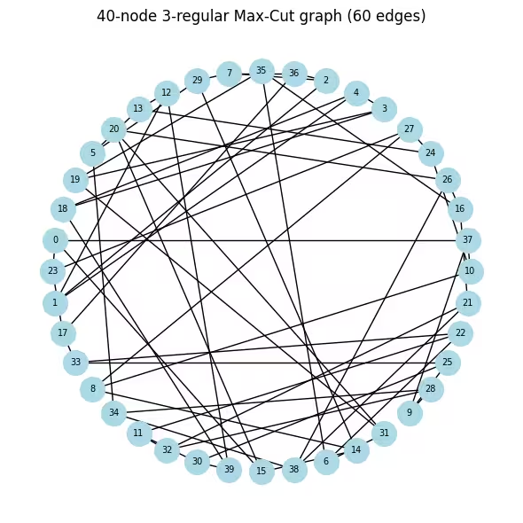
Cost operator: 40 qubits, 60 Pauli terms
c* range: [0.000, 1.000]  theta range: [1.047, 2.094] rad

Transpiled circuit: 2Q depth=86

# ── Classical baseline via simulated annealing ────────────────────
# Run SA before any hardware calls to get a strong classical reference cut
# value. SA is fast (seconds), needs no solver license, and reliably finds
# near-optimal solutions on 40-node graphs. We use sa_cut as the denominator
# for the approximation ratio instead of the looser QP upper bound.
#
# At each step we flip a random node and accept the move if it improves the
# cut, or with probability exp(delta/T) otherwise. Temperature T decays
# geometrically, allowing uphill moves early on to escape local minima.
def simulated_annealing_maxcut(
    G, seed=0, T0=2.0, T_min=1e-4, alpha=0.995, n_steps=100_000
):
    rng_sa = np.random.default_rng(seed)
    n = G.number_of_nodes()
    x = rng_sa.integers(0, 2, n)
    best_x = x.copy()
    best_cut = sum(1 for u, v in G.edges() if x[u] != x[v])
    T = T0
    for _ in range(n_steps):
        i = rng_sa.integers(0, n)
        delta = sum((-1 if x[i] != x[nb] else 1) for nb in G.neighbors(i))
        if delta > 0 or rng_sa.random() < np.exp(delta / T):
            x[i] ^= 1
            cut = sum(1 for u, v in G.edges() if x[u] != x[v])
            if cut > best_cut:
                best_cut, best_x = cut, x.copy()
        T = max(T * alpha, T_min)
    return best_x, best_cut

sa_solution, sa_cut = simulated_annealing_maxcut(G_large)
print(f"Simulated annealing cut value: {sa_cut}  (classical reference)")

# ── Step 3: Execution on hardware ───────────────────────────
# A Session reserves the backend so the COBYLA iterations and final sampling
# run back-to-back without re-queuing between jobs — important when the
# optimizer submits many short jobs sequentially. All jobs are tagged with
# "TUT_WSQAOA" for traceability in the IBM Quantum dashboard.
#
# EstimatorV2 with resilience_level=1 enables twirled readout error extinction
# (TREX), which corrects systematic measurement bit-flip errors without extra
# circuit overhead. 4096 shots per call balances estimation noise vs. job time.
estimator_options = EstimatorOptions()
estimator_options.resilience_level = 1
estimator_options.default_shots = 4096
estimator_options.environment.job_tags = ["TUT_WSQAOA"]

# Align the cost observable with the physical qubit layout chosen by the transpiler
cost_op_isa = cost_op_large.apply_layout(ws_isa_large.layout)
ws_param_order_isa = list(ws_isa_large.parameters)

ws_history_hw = []

with Session(backend=backend) as session:
    estimator_hw = Estimator(mode=session, options=estimator_options)

    def hw_cost_fn(params):
        bound = ws_isa_large.assign_parameters(
            dict(zip(ws_param_order_isa, params))
        )
        energy = (
            estimator_hw.run([(bound, cost_op_isa)]).result()[0].data.evs.real
        )
        ws_history_hw.append(float(energy))
        print(
            f"  iter {len(ws_history_hw):>3d}  <H_C> = {energy:.4f}", end="\r"
        )
        return float(energy)

    # Warm-start initialization: gamma=0 means the cost unitary is the identity on
    # the first call, so COBYLA immediately evaluates the warm-start state itself —
    # a much better starting signal than a random point.
    ws_params0_hw = np.concatenate(
        [np.zeros(p_large), np.full(p_large, np.pi / 4)]
    )

    ws_result_hw = minimize(
        hw_cost_fn,
        ws_params0_hw,
        method="COBYLA",
        options={"maxiter": 150, "rhobeg": 0.3},
    )
    print(
        f"\nOptimization complete: energy={ws_result_hw.fun:.4f}, "
        f"iterations={len(ws_history_hw)}"
    )

    # ── Step 3b: Sample the optimized circuit ──────────────────────────────────
    # Use 8192 shots for the final sample to get a reliable mode estimate.
    sampler_hw = Sampler(
        mode=session,
        options={"environment": {"job_tags": ["TUT_WSQAOA"]}},
    )
    ws_bound_hw = ws_isa_large.assign_parameters(
        dict(zip(ws_param_order_isa, ws_result_hw.x))
    )
    counts_hw = (
        sampler_hw.run([ws_bound_hw], shots=8192)
        .result()[0]
        .data.meas.get_counts()
    )

best_bs_hw = max(counts_hw, key=counts_hw.get)
best_count = counts_hw[best_bs_hw]
total_shots = sum(counts_hw.values())

# Decode: Qiskit returns bitstrings with qubit 0 at the rightmost position,
# so reversing the string maps character index i to variable x_i.
cut_val_hw, s0_hw, s1_hw = evaluate_cut(best_bs_hw[::-1], G_large)

# Compare against simulated annealing.
# A ratio >= 1.0 means WS-QAOA matched or beat the classical SA solution.
# A ratio close to 1.0 (e.g. > 0.95) shows the quantum result is competitive.
approx_ratio_hw = cut_val_hw / sa_cut
print(
    f"Most-probable bitstring frequency: {best_count}/{total_shots} "
    f"({100*best_count/total_shots:.1f}%)"
)
print(
    f"WS-QAOA cut: {cut_val_hw}  |  SA cut: {sa_cut}  "
    f"|  Approximation ratio vs SA: {approx_ratio_hw:.4f}"
)

# Visualize both solutions side-by-side on the graph.
# Blue = partition S, orange = partition S-bar.
# Edges crossing between colors are the ones counted in the cut.
fig, axes = plt.subplots(1, 2, figsize=(14, 6))
for ax, assignment, cut, title in [
    (
        axes[0],
        list(sa_solution),
        sa_cut,
        f"Simulated Annealing (cut={sa_cut})",
    ),
    (
        axes[1],
        [int(b) for b in best_bs_hw[::-1]],
        cut_val_hw,
        f"WS-QAOA hardware (cut={cut_val_hw})",
    ),
]:
    colors = [
        "skyblue" if assignment[i] == 0 else "salmon" for i in G_large.nodes()
    ]
    nx.draw(
        G_large,
        pos_large,
        with_labels=True,
        node_color=colors,
        node_size=400,
        font_size=7,
        ax=ax,
    )
    ax.set_title(title)
plt.suptitle("Max-Cut partitions: SA vs WS-QAOA", fontsize=13)
plt.tight_layout()
plt.show()

# ── Step 4: Convergence plot and summary ──────────────────────────────────
# On real hardware the trace will be noisy (shot noise + gate errors), but the
# overall downward trend confirms that COBYLA is making progress despite noise.
fig, ax = plt.subplots(figsize=(7, 4))
ax.plot(ws_history_hw, color="tab:orange", label="WS-QAOA (hardware)")
ax.axhline(
    ws_result_hw.fun,
    color="tab:orange",
    linestyle=":",
    label=f"Final energy ({ws_result_hw.fun:.3f})",
)
ax.set_xlabel("Optimizer call")
ax.set_ylabel(r"$\langle H_C \rangle$")
ax.set_title(f"WS-QAOA convergence on {backend.name} (40 qubits, p=1)")
ax.legend()
plt.tight_layout()
plt.show()

print("\n=== Large Scale Summary ===")
print(f"{'Metric':<38} {'Value':>10}")
print("-" * 50)
print(f"{'Nodes / Edges':<38} {N_LARGE:>5} / {len(edges_large):<4}")
print(f"{'QAOA layers (p)':<38} {p_large:>10}")
print(f"{'Transpiled ECR gate count':<38} {ecr_count:>10}")
print(f"{'Transpiled circuit depth':<38} {ws_isa_large.depth():>10}")
print(f"{'Optimizer iterations':<38} {len(ws_history_hw):>10}")
print(f"{'WS-QAOA energy (hardware)':<38} {ws_result_hw.fun:>10.4f}")
print(f"{'Cut value':<38} {cut_val_hw:>10}")
print(f"{'Simulated annealing cut value':<38} {sa_cut:>10}")
print(f"{'Approximation ratio (vs SA)':<38} {approx_ratio_hw:>10.4f}")

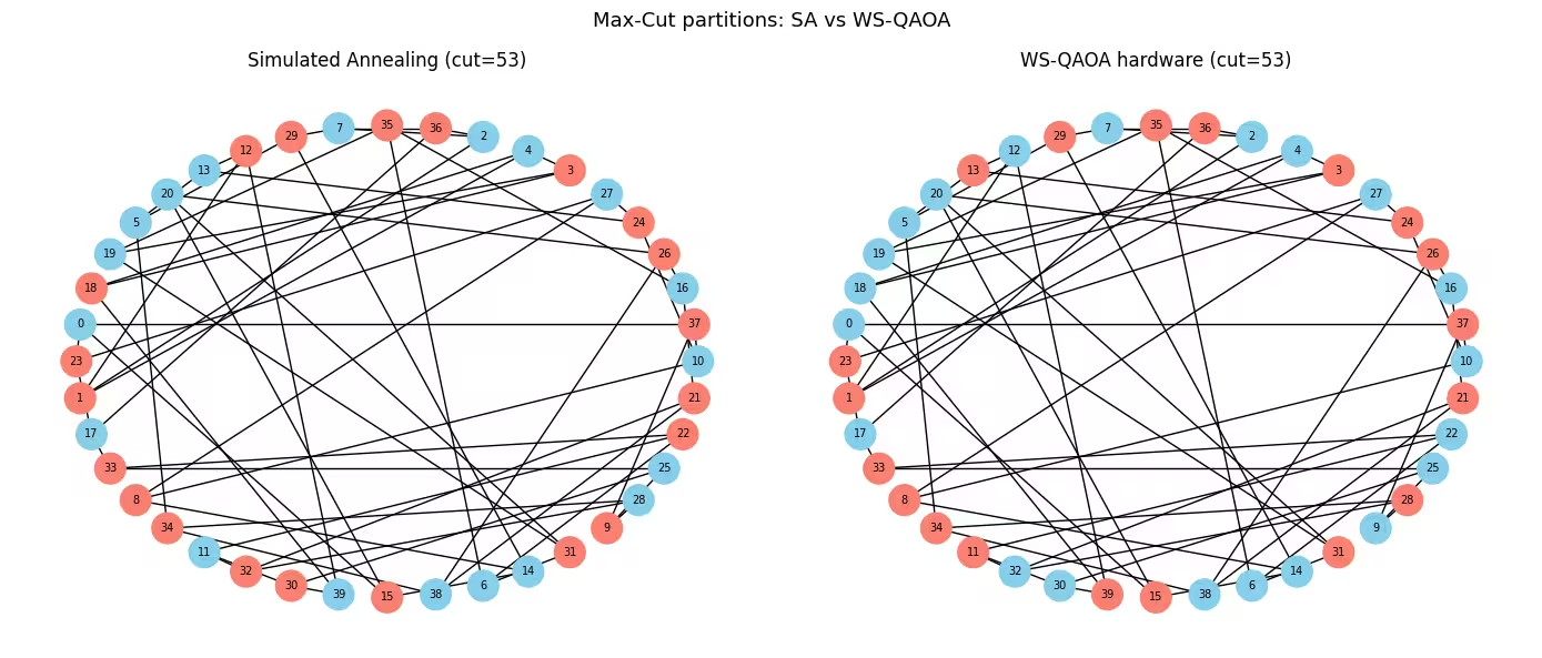
Simulated annealing cut value: 53  (classical reference)
  iter  31  <H_C> = -12.4094
Optimization complete: energy=-13.0256, iterations=31
Most-probable bitstring frequency: 4/8192 (0.0%)
WS-QAOA cut: 53  |  SA cut: 53  |  Approximation ratio vs SA: 1.0000

=== Large Scale Summary ===
Metric                                      Value
--------------------------------------------------
Nodes / Edges                             40 / 60  
QAOA layers (p)                                 1
Transpiled ECR gate count                       0
Transpiled circuit depth                      276
Optimizer iterations                           31
WS-QAOA energy (hardware)                -13.0256
Cut value                                      53
Simulated annealing cut value                  53
Approximation ratio (vs SA)                1.0000

Kolejne kroki

Rekomendacje

Jeśli ta praca wydała ci się interesująca, możesz zainteresować się następującymi materiałami:

• Więcej warstw QAOA: Zwiększ p, aby zobaczyć, jak oba algorytmy poprawiają się wraz z większą liczbą warstw obwodu, i czy przewaga WS-QAOA przy niskiej głębokości się utrzymuje.
• Dodatek Qiskit optimization mapper: Zapoznaj się z dokumentacją i spróbuj modelować różne problemy kombinatoryczne lub używać różnych solverów dla relaksacji ciągłej.

Odnośniki

[1] D. J. Egger, J. Mareček, and S. Woerner, "Warm-starting quantum optimization," Quantum, vol. 5, p. 479, 2021. arXiv:2009.10095

[2] E. Farhi, J. Goldstone, and S. Gutmann, "A quantum approximate optimization algorithm," arXiv:1411.4028, 2014.